taylor-polynomial

A finite polynomial that locally approximates a smooth function around a chosen point. The Taylor polynomial of degree $n$ matches the function’s value and first $n$ derivatives at that point, making it useful for analytical and numerical reasoning about local behaviour.

Why Polynomials?

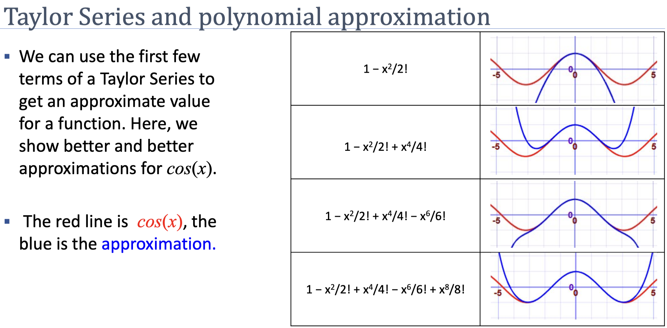
Taylor approximation has a supremely practical goal: take a complicated, non-polynomial function like $\cos (x)$ or $e^x$ and replace it locally with a polynomial that behaves the same way.

Why polynomials? Because they are the friendliest tools we have. Polynomials are easy to compute (just additions and multiplications), easy to differentiate, and easy to integrate. Replacing a hard function with a polynomial that matches it near a chosen point turns intractable analysis into algebra.

The fundamental intuition: you translate derivative information at a single point into approximation information around that point. Every twist of the function at the centre — its value, slope, curvature, rate of change of curvature, and so on — is encoded into a single coefficient of the polynomial. Match enough derivatives and the polynomial mimics the function.

Definition

The Taylor polynomial of degree $n$ of a function $f$ around the point $a$ is:

$T_n(x)={\sum }_{k=0}^n\frac{f^{(k)}(a)}{k!}(x-a{)}^k$

where $f^{(k)}(a)$ is the $k$-th derivative of $f$ evaluated at $a$.

Expanding the first few terms:

$T_n(x)=f(a)+f^{\prime }(a)(x-a)+\frac{f^{\prime \prime }(a)}{2!}(x-a{)}^2+\frac{f^{\prime \prime \prime }(a)}{3!}(x-a{)}^3+\cdots$

The infinite series (taking $n\to \infty$) is the Taylor series; for analytic functions it equals $f$ exactly within some radius of convergence.

Coefficients as Independent Derivative Controls

Forget the formula for a moment and write a generic polynomial centred at $a$:

$T(x)=c_0+c_1(x-a)+c_2(x-a{)}^2+c_3(x-a{)}^3+\cdots$

The coefficients $c_0,c_1,c_2,\dots$ are free parameters — we get to choose them. The Taylor expansion picks each one so that it controls exactly one derivative of $T$ at $a$, independently of all the others:

• $c_0$ controls the value at $x=a$. Plug $x=a$ into $T$ and every $(x-a)$ term vanishes, leaving $T(a)=c_0$. To match the function, set $c_0=f(a)$.
• $c_1$ controls the first derivative (slope) at $a$. Differentiate once: $T^{\prime }(x)=c_1+2c_2(x-a)+3c_3(x-a{)}^2+\cdots$. Plug in $x=a$ and only $c_1$ survives: $T^{\prime }(a)=c_1$. Set $c_1=f^{\prime }(a)$.
• $c_2$ controls the second derivative (curvature) at $a$. Differentiate twice: $T^{\prime \prime }(x)=2c_2+6c_3(x-a)+\cdots$. At $x=a$, only $c_2$ contributes: $T^{\prime \prime }(a)=2c_2$.
• $c_n$ generally controls the $n$-th derivative at $a$.

The independence is the magic: when you take $k$ derivatives and evaluate at $x=a$, every term of degree higher than $k$ still contains an $(x-a)$ factor and vanishes. So matching the $k$-th derivative locks in $c_k$ alone, without disturbing any other coefficient. We can build the approximation derivative-by-derivative.

Why the $n!$?

The factorial in the denominator is the price of the power rule. Watch what happens to $(x-a{)}^4$ as you differentiate it repeatedly:

Step	Result
$(x-a{)}^4$	$(x-a{)}^4$
First derivative	$4(x-a{)}^3$
Second	$4\cdot 3(x-a{)}^2$
Third	$4\cdot 3\cdot 2(x-a)$
Fourth	$4\cdot 3\cdot 2\cdot 1=4!$

Each differentiation peels off a power and multiplies in a new integer. After $n$ derivatives of $(x-a{)}^n$ you are left with $n!$ — a constant. So $T_n^{(n)}(a)=n!c_n$, not just $c_n$.

To make $T_n^{(n)}(a)$ equal $f^{(n)}(a)$, we have to divide out the $n!$ that the power rule manufactures:

$c_n=\frac{f^{(n)}(a)}{n!}$

The factorial isn’t decoration — it is a correction factor that cancels the cascading multiplicative effect of repeated differentiation.

Geometric Interpretation by Degree

Degree	Captures	Geometry
$0$	Value at $a$	Constant $f(a)$ — flat horizontal line
$1$	Value + slope	Tangent line at $a$
$2$	Value + slope + curvature	Tangent parabola
$\ge 3$	Higher-order shape	Increasingly accurate near $a$

A degree-1 Taylor polynomial says “approximate the function with its tangent line.” A degree-2 says “approximate it with the parabola that matches value, slope, and curvature.” Higher degrees match progressively more derivatives.

The Approximation Is Local

Taylor polynomials are accurate near the centre $a$ and degrade as $|x-a|$ grows. A degree-2 approximation of $\cos (x)$ around $0$ matches well in $(-\pi /4,\pi /4)$ but is hopeless at $x=\pi$.

You can tighten the approximation by either:

• Increasing the degree $n$ — more derivatives matched, more terms.
• Re-centring at a closer point — pick $a$ near the $x$ of interest.

Many iterative algorithms (including Newton-Raphson) lean on the second strategy: they re-build a low-degree Taylor approximation around the current iterate and step toward its optimum.

Convergence and the Radius of Convergence

The Taylor polynomial uses finitely many terms. The Taylor series takes the limit $n\to \infty$. Whether that infinite sum equals the original function depends on the function and the chosen centre:

• Convergence: as you add terms, the partial sums get arbitrarily close to a finite value. For $e^x$ centred at $0$, the series converges to $e^x$ for every real $x$, no matter how far from $0$. Smooth functions whose higher derivatives stay tame behave this way.
• Divergence: adding terms fails to approach anything. Partial sums oscillate or blow up.
• Radius of convergence: many functions sit in between. The series converges for inputs within a fixed distance $R$ of the centre and diverges beyond it. $R$ is the radius of convergence.

A canonical mid-case is $\ln (x)$ centred at $a=1$. Its Taylor series converges only on $(0,2)$ — a radius of $1$. At $x=0$ the function blows up to $-\infty$, and the series cannot reach across that singularity even though derivative information at $a=1$ is perfectly well-defined. Beyond $x=2$ the series diverges in the symmetric direction.

ASIDE — A map of a single street corner

Think of the derivative information at $a$ as an extremely detailed map of a single street corner — the slope, the curvature, the rate of change of curvature, every higher-order twist. A Taylor polynomial uses that map to mimic the function’s behaviour right around $a$. If the function is smooth enough (like $e^x$), the local map accurately guides you across the entire real line. But if there is complicated behaviour nearby (like the singularity of $\ln (x)$ at $0$), the map only helps for a finite distance — beyond that, the approximation fails and the series spins out of control.

For optimisation purposes, convergence properties matter much less than for analysis. Algorithms like Newton-Raphson take a single step from the current iterate’s quadratic approximation and then re-centre — they never push the approximation out toward its radius of convergence, so divergence never has a chance to bite.

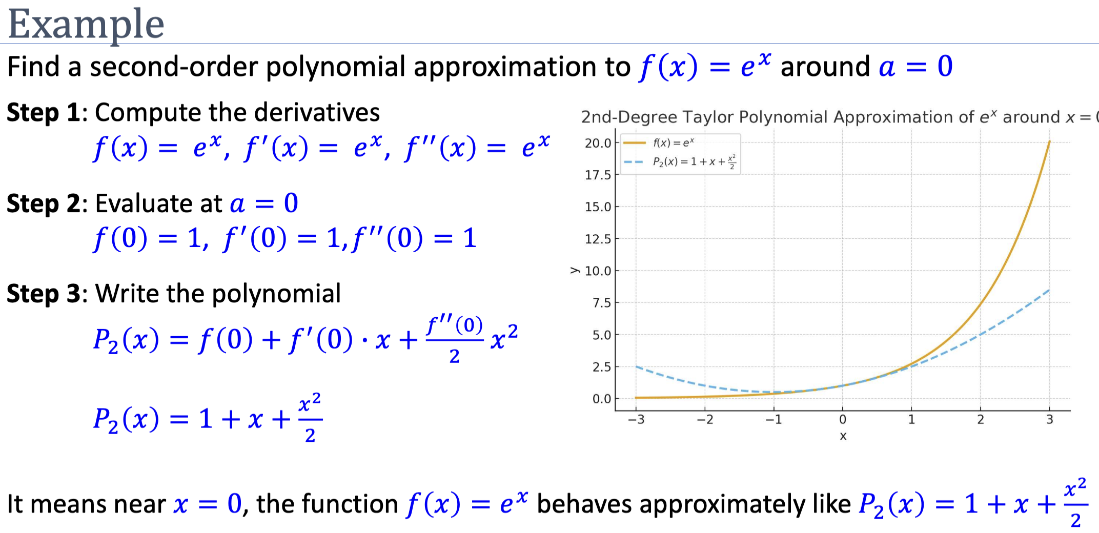
Worked Example: $e^x$ Around $0$

For $f(x)=e^x$, all derivatives are $e^x$, so $f^{(k)}(0)=1$ for every $k$. The degree-$n$ Taylor polynomial is:

$T_n(x)={\sum }_{k=0}^n\frac{x^k}{k!}=1+x+\frac{x^2}{2}+\frac{x^3}{6}+\cdots +\frac{x^n}{n!}$

The degree-2 approximation $P_2(x)=1+x+x^2/2$ is very close to $e^x$ for $|x|<1$, fair for $|x|<2$, poor beyond.

Use in Optimisation

The degree-2 Taylor polynomial of a loss $E(w)$ around the current iterate $w_0$ is:

$T_2(w)=E(w_0)+(w-w_0)E^{\prime }(w_0)+\frac{(w-w_0{)}^2}{2}{E}^{\prime \prime }(w_0)$

This is a parabola — and a parabola has a closed-form minimum. Setting $T_2^{\prime }(w)=0$ gives:

$E^{\prime }(w_0)+(w-w_0)E^{\prime \prime }(w_0)=0⟹w=w_0-\frac{E^{\prime }(w_0)}{E^{\prime \prime }(w_0)}$

This is the Newton-Raphson update. The algorithm replaces the true loss with its quadratic Taylor approximation, jumps to the parabola’s minimum, then re-approximates around the new point. The multivariate generalisation involves the Hessian.

gradient descent can also be derived from a Taylor view: it corresponds to using a degree-1 Taylor approximation plus a fixed step constraint. Because a linear approximation has no minimum (it’s a line), the algorithm needs an externally-supplied step size — the learning rate.

Related

• newton-raphson-method — uses a degree-2 Taylor approximation
• hessian-matrix — the multivariate analogue of $f^{\prime \prime }(a)$
• gradient descent — corresponds (loosely) to a degree-1 Taylor view

Active Recall

Find the second-order Taylor polynomial of $f(x)=e^x$ around $a=0$.

$f(x)=e^x$, $f^{\prime }(x)=e^x$, $f^{\prime \prime }(x)=e^x$. At $a=0$: $f(0)=f^{\prime }(0)=f^{\prime \prime }(0)=1$. So $P_2(x)=1+x+x^2/2$. Near $x=0$, $e^x$ behaves approximately like this parabola.

Why does the degree-2 Taylor polynomial of a loss function lead naturally to an optimisation update rule, while the degree-1 polynomial does not?

A degree-2 polynomial is a parabola — it has a unique minimum (when curvature is positive) at a closed-form location, derivable by setting its derivative to zero. The optimiser jumps directly there. A degree-1 polynomial is a line, which has no minimum. So the algorithm using a degree-1 view needs an external step size — the learning rate of gradient descent — because it can’t determine “how far to go” from the approximation alone.

Why are Taylor approximations only accurate locally?

The polynomial matches $f$‘s value and derivatives at the centre $a$, so the two functions agree exactly there. As you move away, higher derivatives that the polynomial doesn’t match start to dominate the difference. Functions whose higher derivatives grow rapidly (like $\sin$, $\cos$, $1/(1-x)$ near $x=1$) lose accuracy quickly; functions whose derivatives stay bounded ($e^x$ near 0, polynomials) approximate well over wider intervals.

Why is the coefficient of $(x-a{)}^4$ in a Taylor polynomial $f^{(4)}(a)/4!$ rather than simply $f^{(4)}(a)$?

Differentiating $(x-a{)}^4$ four times produces a cascade: $4(x-a{)}^3$, then $4\cdot 3(x-a{)}^2$, then $4\cdot 3\cdot 2(x-a)$, then $4\cdot 3\cdot 2\cdot 1=24=4!$. So the fourth derivative of $c_4(x-a{)}^4$ at $x=a$ is $4!c_4$, not $c_4$. Setting that equal to $f^{(4)}(a)$ requires $c_4=f^{(4)}(a)/4!$. The factorial cancels the multiplicative effect that the power rule manufactures during repeated differentiation.

Why does each Taylor coefficient control exactly one derivative of the polynomial at the centre, independently of the others?

When you take $k$ derivatives of $T(x)={\sum }_n{c}_n(x-a{)}^n$ and evaluate at $x=a$, every term of degree higher than $k$ still contains an $(x-a)$ factor and vanishes; every term of degree below $k$ has been differentiated to zero already; only the degree-$k$ term contributes. So $T^{(k)}(a)$ depends on $c_k$ alone. This is what lets us build the polynomial derivative-by-derivative — fixing $c_k$ to match $f^{(k)}(a)$ doesn’t disturb any earlier or later coefficient.

The Taylor series for $\ln (x)$ centred at $a=1$ has radius of convergence $1$. Why doesn't it extend further?

$\ln (x)$ has a singularity at $x=0$, where it diverges to $-\infty$. The radius of convergence cannot reach across a singularity — the derivative information collected at $a=1$ “doesn’t propagate” beyond it. So the series converges on $(0,2)$ — distance $1$ in either direction from the centre — and diverges outside. Functions like $e^x$ have no singularities anywhere on $\mathbb{R}$, so their Taylor series converge for every real input.