gradient-descent-ml

A first-order iterative optimisation algorithm: from any starting point, repeatedly step in the direction of the negative gradient, scaled by a learning rate. The workhorse of machine learning optimisation.

The Algorithm

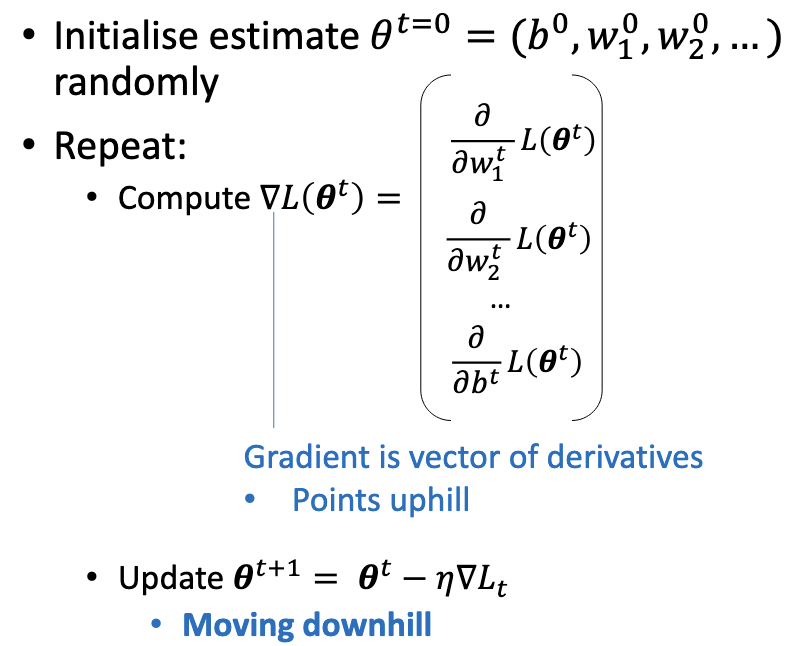
To minimise a differentiable function $E(\mathbf{w})$:

1. Initialise $\mathbf{w}$ (often zeros or small random values).
2. Repeat until convergence: $\mathbf{w}\leftarrow \mathbf{w}-\eta \nabla E(\mathbf{w})$

The hyperparameter $\eta >0$ is the learning rate. Convergence is typically declared when $\Vert \nabla E(\mathbf{w})\Vert$ falls below a threshold or after a fixed number of iterations.

Why It Works

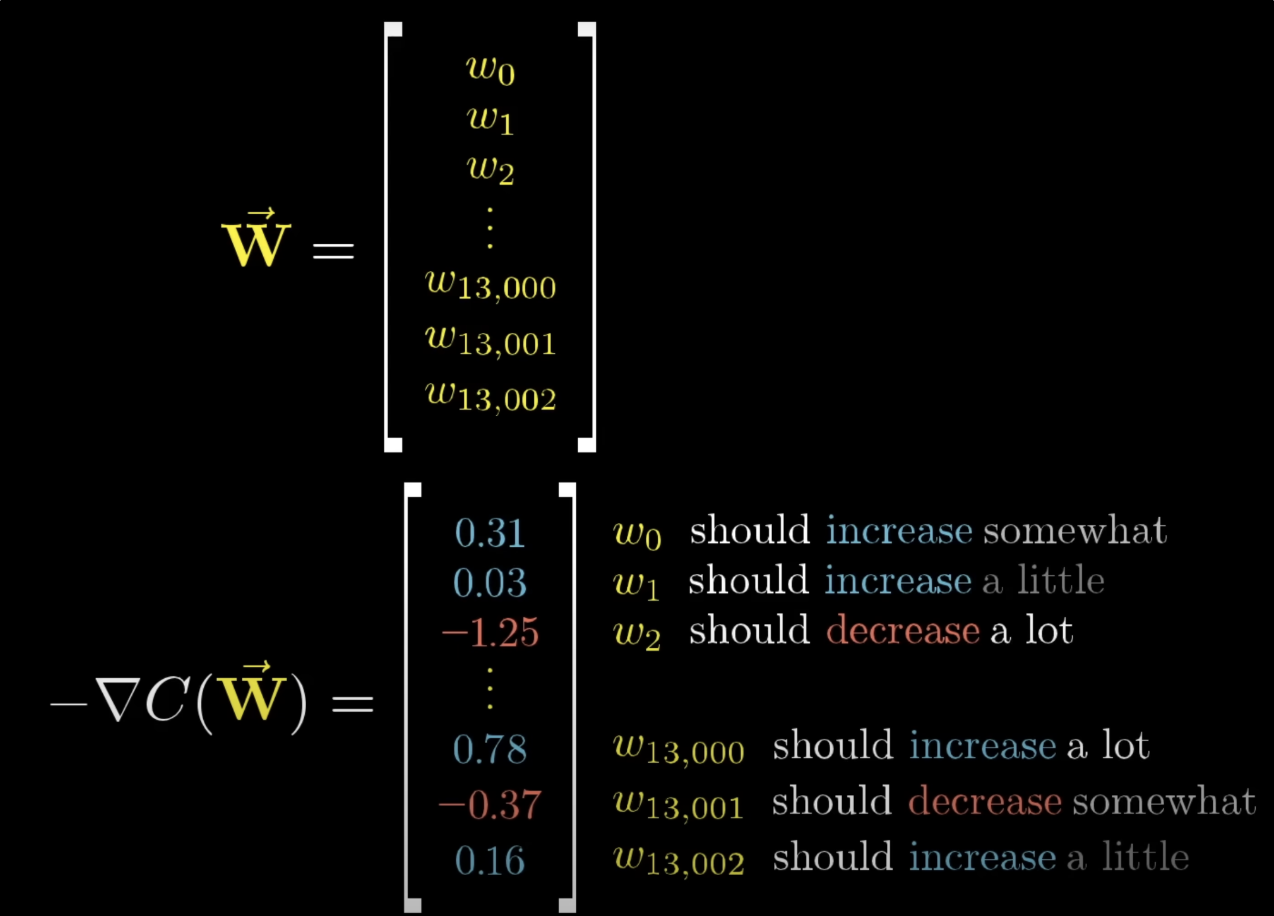
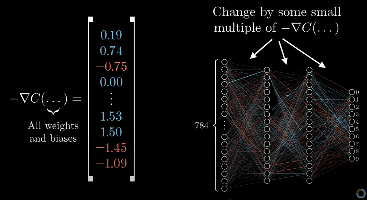
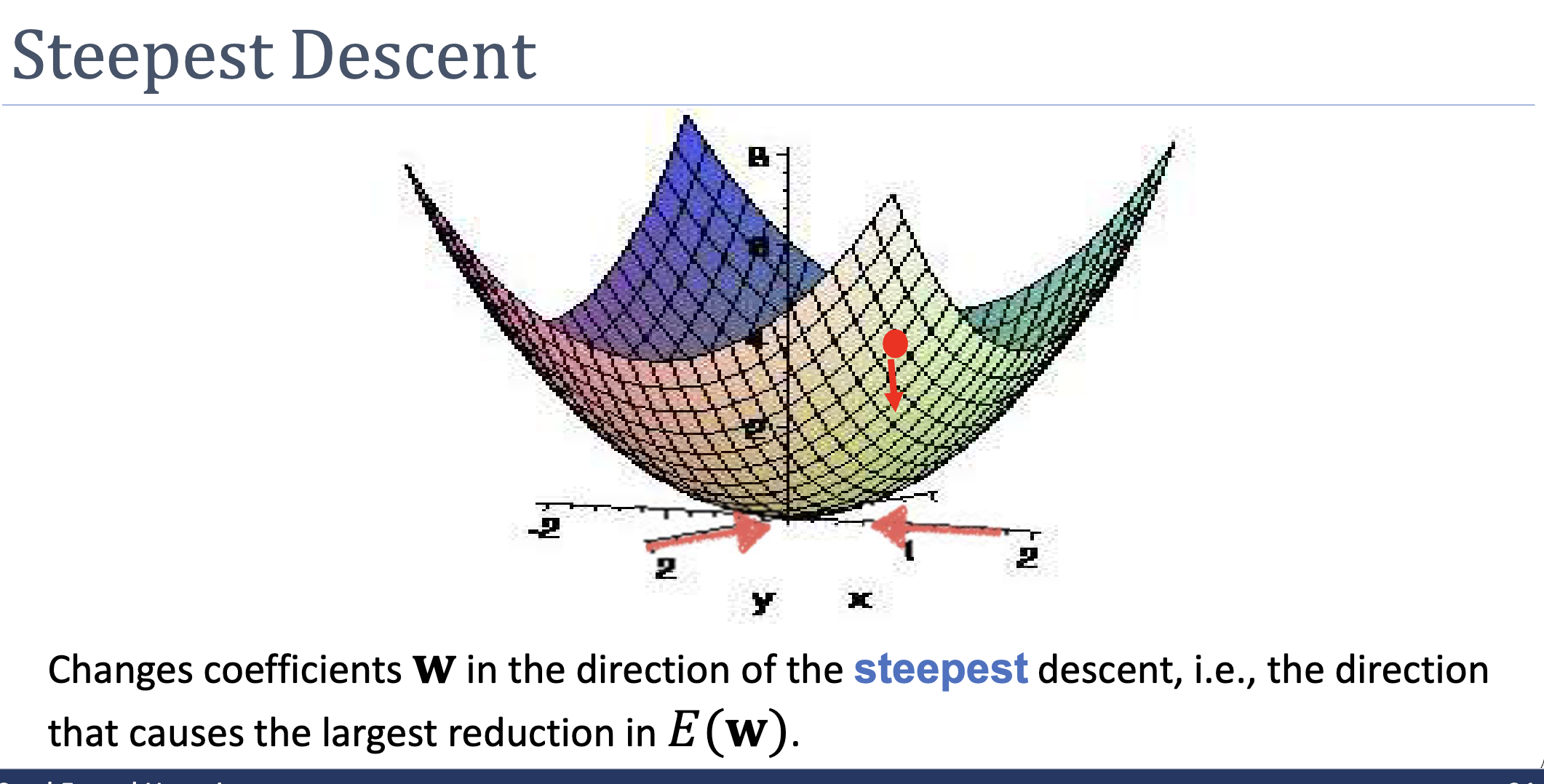
The gradient $\nabla E(\mathbf{w})$ is the vector of partial derivatives, pointing in the direction of steepest increase of $E$. The negative gradient points in the direction of steepest decrease. By the definition of the derivative, for a small enough step in that direction, $E$ is guaranteed to decrease.

The qualifier “small enough” is critical. The negative gradient is the steepest direction instantaneously; over a finite step it may overshoot the minimum or move into a region where the gradient itself has changed substantially.

The Learning Rate Trade-off

Picking $\eta$ is a balancing act:

• Too large: each step jumps past the minimum, possibly landing on the opposite slope at higher loss. Iterations bounce around or diverge.
• Too small: each step moves a negligible distance. Convergence still happens but takes prohibitively many iterations.

There is no universally right $\eta$ — it depends on the curvature of $E$. Practically, one tries a few values (e.g., $0.1,0.01,0.001$), watches the loss curve, and adjusts. More sophisticated schemes (decay schedules, line search, adaptive methods like Adam) handle this dynamically.

Differential Curvature: The Achilles Heel

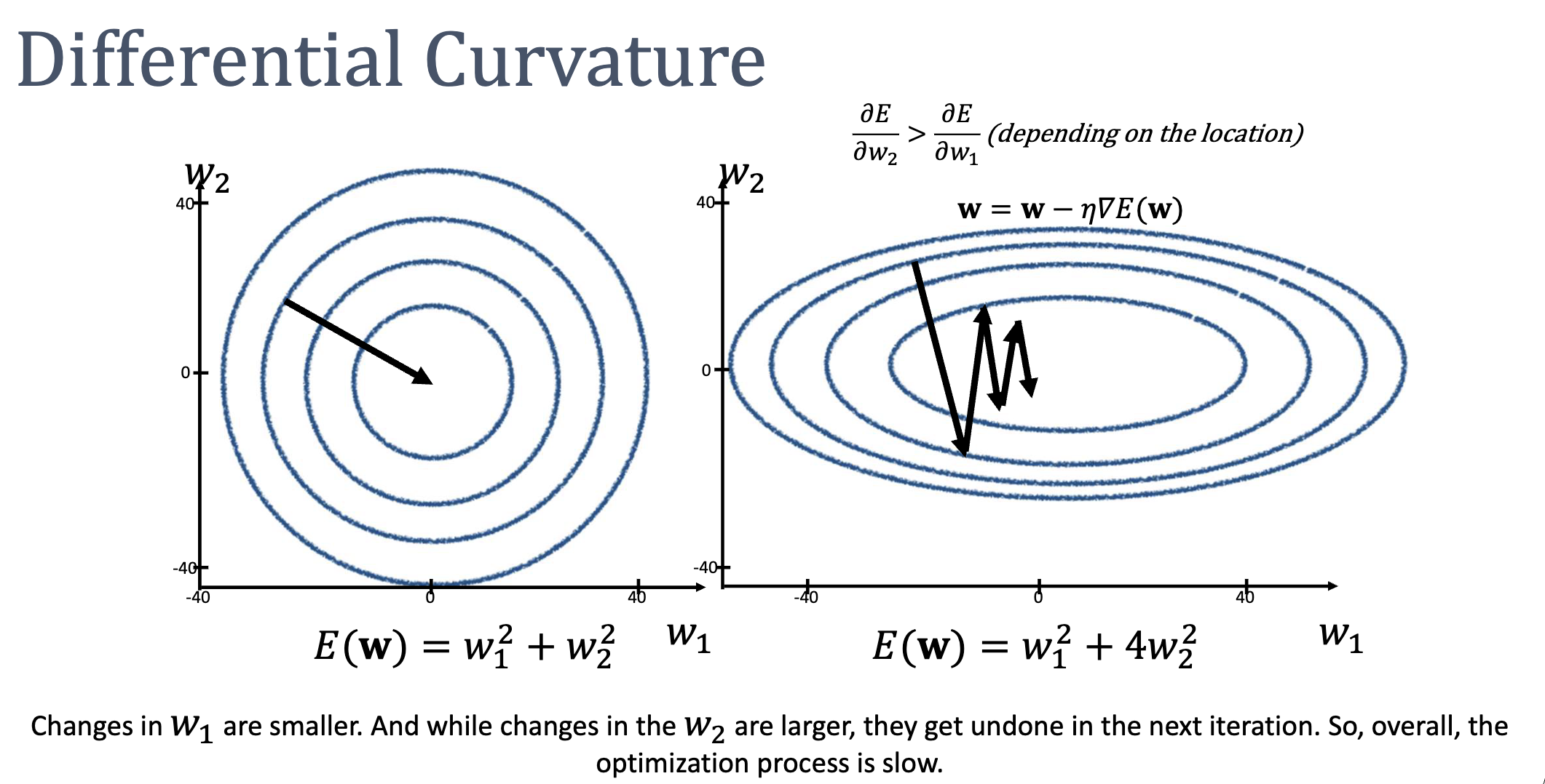
The same $\eta$ scales every dimension of the update. This breaks down badly when different weights have different curvature — i.e., the loss surface is shaped like a long narrow valley rather than a round bowl.

Consider $E(\mathbf{w})=w_1^2+4w_2^2$. The contours are ellipses, with $w_2$ four times steeper than $w_1$. Gradient descent’s path zigzags across the narrow direction while creeping slowly along the long direction:

• Set $\eta$ small enough to avoid overshooting in $w_2$ → $w_1$ updates become tiny.
• Set $\eta$ large enough to make progress in $w_1$ → $w_2$ overshoots and bounces.

The fundamental problem: gradient descent uses only first-order (slope) information. It has no idea how the slope itself is changing across the surface.

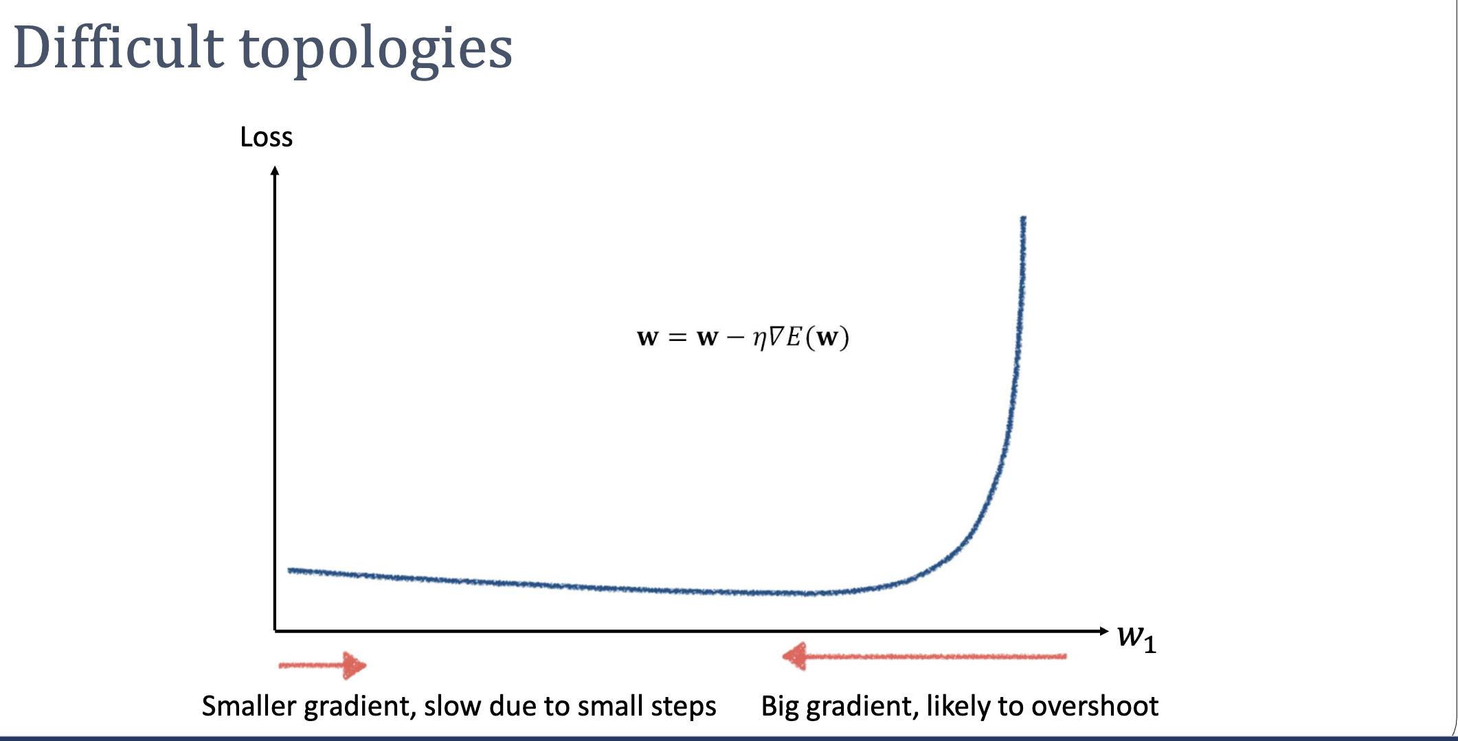
The same pathology shows up in 1D when the loss is shallow on one side and explodes on the other — a single $\eta$ can’t be both large enough for the flat region and small enough for the steep one:

ASIDE — Standardisation helps but isn't a cure

Standardising input features (zero mean, unit variance) often reshapes the loss surface from ellipses toward circles, mitigating curvature mismatch. But the loss landscape’s geometry is shaped by feature interactions and the loss function’s structure, not just feature scales — so standardisation alleviates the issue without eliminating it. To actually adapt to local curvature, you need a second-order method like Newton-Raphson.

Local Minima

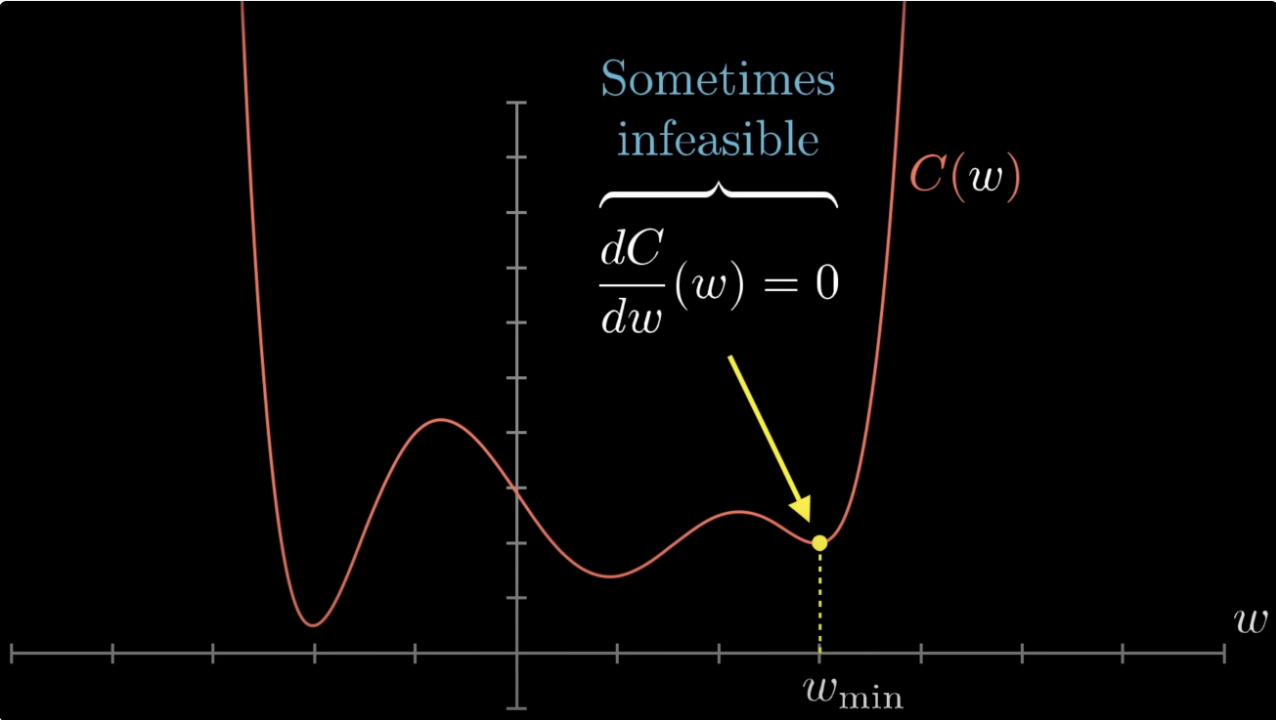
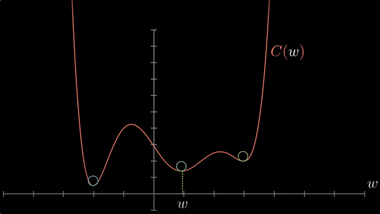
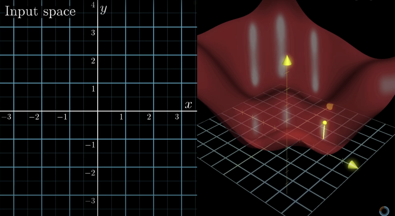
Gradient descent finds a critical point (where $\nabla E=0$), not necessarily the global minimum. On non-convex losses (e.g., neural networks), it can get stuck in local minima or saddle points.

For convex losses, this isn’t a worry: every local minimum is a global minimum. The cross-entropy-loss for logistic-regression is strictly convex in $\mathbf{w}$, so gradient descent that converges to a critical point converges to the unique global optimum.

Steepest Descent Is Only Locally Optimal

The negative gradient is the direction of steepest descent at the current point. It is not guaranteed to be the best direction over a longer trajectory. In a long narrow valley, the best direction is along the valley toward the minimum, but the steepest direction at most points is roughly perpendicular to the valley (pointing toward the closer wall). This mismatch is why gradient descent zigzags.

The Update Rule for Logistic Regression

For logistic-regression with cross-entropy-loss:

$\nabla E(\mathbf{w})={\sum }_{i=1}^N(p_1({\mathbf{x}}^{(i)},\mathbf{w})-y^{(i)}){\mathbf{x}}^{(i)}$

so the gradient descent update is:

$\mathbf{w}\leftarrow \mathbf{w}-\eta {\sum }_{i=1}^N(p_1({\mathbf{x}}^{(i)},\mathbf{w})-y^{(i)}){\mathbf{x}}^{(i)}$

Each step requires summing over the entire training set — this is batch gradient descent. Variants include stochastic (one example per step) and mini-batch (a subset per step), trading update accuracy for speed.

Related

• cross-entropy-loss — the loss gradient descent typically minimises for logistic regression
• newton-raphson-method — second-order alternative that adapts step size to curvature
• convex-function — the property that lets gradient descent succeed reliably
• taylor-polynomial — gradient descent corresponds to using a degree-1 Taylor approximation

Active Recall

Suppose the loss surface has very different curvatures along different axes. What pathological behaviour will gradient descent exhibit, and why does standardising input features only partially fix it?

Gradient descent zigzags: large gradient components along the high-curvature axes cause overshooting and bouncing, while small components along the low-curvature axes produce glacially slow progress along the valley toward the minimum. Standardising features rescales them to similar magnitudes, which often makes the loss surface more isotropic — but the curvature of the loss is determined by feature interactions and the loss function’s structure, not just feature scales. To genuinely adapt to local curvature, you need second-order information (the Hessian).

Why is gradient descent guaranteed to find the global minimum of the cross-entropy loss for logistic regression but not, in general, for a neural network?

The cross-entropy loss for logistic regression is strictly convex in $\mathbf{w}$, so it has a unique global minimum and any critical point is that minimum. A neural network’s loss is non-convex in its parameters (because the network is a non-convex function of its weights), so gradient descent can converge to local minima or saddle points that are not the global optimum.

Walk through one gradient descent iteration on $E(w)=w^2$ with starting point $w^{(0)}=-4$ and $\eta =0.8$. What does this illustrate about choosing $\eta$ poorly?

$E^{\prime }(w)=2w$, so $E^{\prime }(-4)=-8$. Update: $w^{(1)}=-4-0.8\cdot (-8)=-4+6.4=2.4$. The next gradient is $E^{\prime }(2.4)=4.8$, so $w^{(2)}=2.4-0.8\cdot 4.8=2.4-3.84=-1.44$. The iterations oscillate around the optimum at $w=0$ rather than converging monotonically. This is the symptom of a learning rate that is large relative to the curvature: progress happens, but with overshoot. (At $\eta =1$ we would oscillate forever; at $\eta >1$ we would diverge.)