Unsupervised Learning: Autoencoders, Representation Learning, Contrastive Learning

THE CRUX: Labelled data is rare and expensive; raw data is abundant. How do we get a network to learn anything useful from images alone, with no labels — and once it has, how do we know the representation is any good?

The whole week is one long answer: design a learning task whose target is the data itself, then judge the resulting representation by how well it solves downstream problems. Three flavours: autoencoders (target = reconstruct your own input through a bottleneck), pretext tasks (target = a label you fabricate from the data, like “where does this patch sit relative to that one?”), and contrastive learning (target = “two augmentations of the same image should land closer in feature space than two unrelated images”). The thread tying them together is representation learning — none of the proxy tasks matter intrinsically; what matters is the encoder you keep at the end.

Where we left off

Week 5 closed the supervised-CNN story: the architecture works, the bag of tricks (init, batch norm, residual, augmentation, dropout, transfer learning) makes it train deeply and generalise, and U-Net showed the encoder-decoder pattern for dense prediction. Every one of those techniques still assumes labelled $(x,y)$ pairs.

This week breaks that assumption. The encoder-decoder shape recurs — autoencoders look superficially like U-Net — but the training signal is no longer a human-supplied label. The data has to supervise itself.

Supervised vs. unsupervised: the framing shift

Supervised learning maps $f_{\theta }:\mathcal{X}\to \mathcal{Y}$ from labelled pairs. The cost: every label needs a human, often an expert (radiologists for medical imaging, drivers for street-scene segmentation). Annotated datasets stay small because labels are the bottleneck.

Unsupervised learning maps $f_{\varphi }:\mathcal{X}\to \mathcal{Z}$ — input only, no $y$. The promise is enormous: 500M tweets a day, billions of unlabelled images, all training fuel for free. The catch is structural — without a $y$, what is the loss? You can’t measure “how wrong” the encoder is when there’s nothing to compare its output against.

TIP — Why it's possible at all

Real images are an absurdly thin slice of pixel-space. A $28\times 28$ greyscale image has $256^{784}\approx 10^{1888}$ possible configurations — more than atoms in the universe ($10^{80}$). Random pixel grids look like static; meaningful images (digits, faces, cats) are a vanishingly small island in that ocean. Data has structure. Unsupervised learning is the search for that structure — find the manifold of “real” images, ignore the noise.

Autoencoders: self-supervision via reconstruction

An autoencoder solves the no-label problem with a trick: make the input itself the target.

• Encoder $f_{\varphi }:\mathcal{X}\to \mathcal{Z}$ compresses $x$ into a code $z$ — the latent-representation (or latent code). “Latent” means hidden: $z$ is an internal vector the network builds en route from $x$ to $\hat{x}$, not directly observed but extractable. The kept deliverable of the AE.
• Decoder $g_{\theta }:\mathcal{Z}\to \mathcal{X}$ reconstructs $\hat{x}=g_{\theta }(f_{\varphi }(x))$.
• Loss is just MSE between input and reconstruction: ${\mathcal{L}}_{rec}=\frac{1}{d}{\sum }_{j=1}^d(x^{(j)}-{\hat{x}}^{(j)}{)}^2$

The data supervises itself. Now there’s a target ($x$), an output ($\hat{x}$), an error, a gradient — the encoder can be trained.

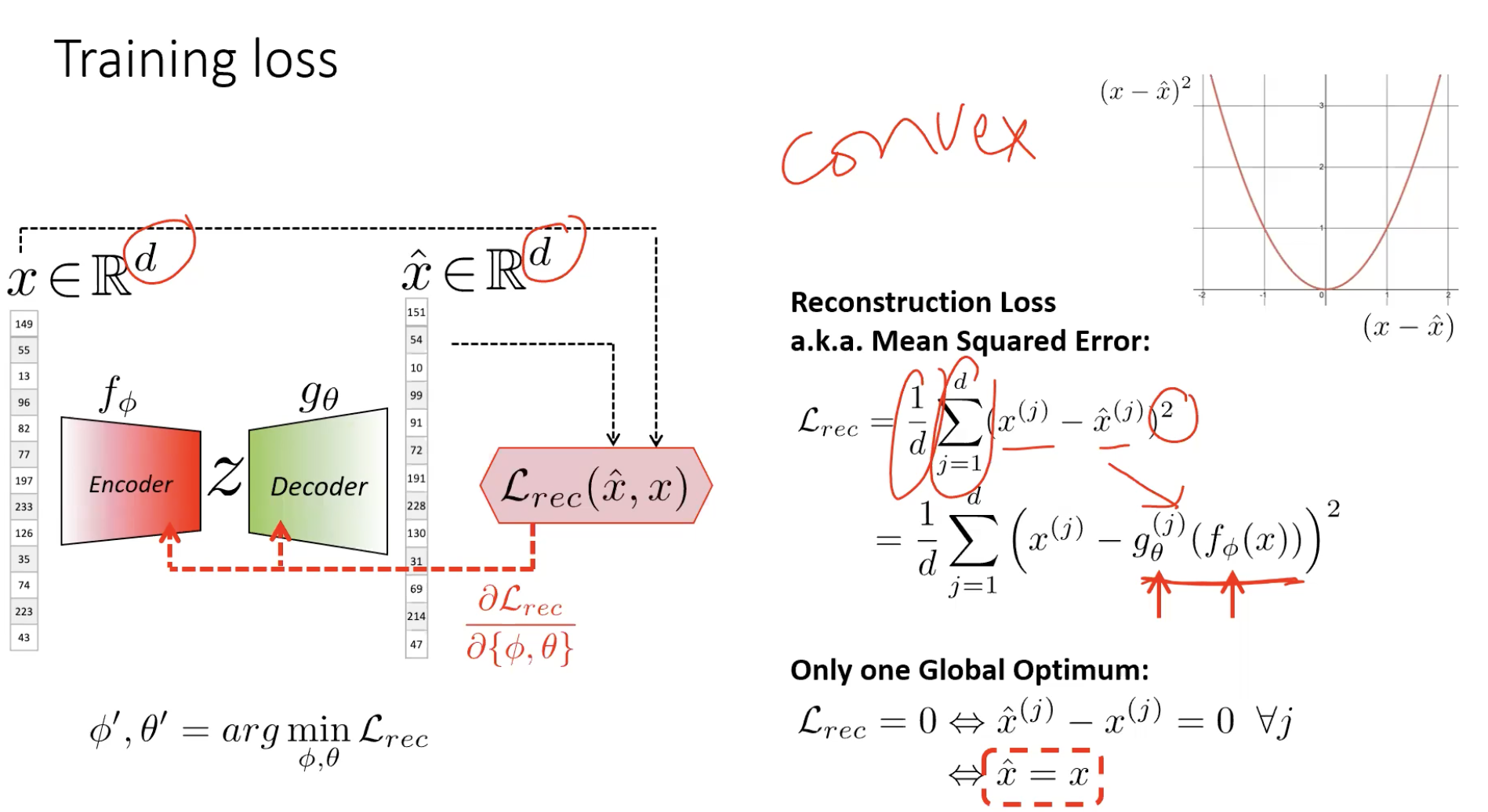
The trivial-solution trap

The loss is minimised when $\hat{x}=x$ — the autoencoder is rewarded for learning the identity function. If $z$ has the same dimensionality as $x$ (or more), the network simply learns $f_{\varphi }(x)=x$ and $g_{\theta }(z)=z$. Loss zero, representation useless.

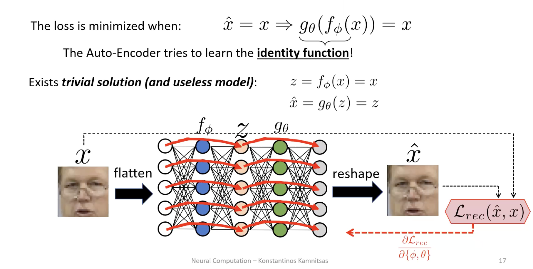
The fix: bottleneck

Force $\dim (\mathcal{Z})=v<d=\dim (\mathcal{X})$. Now the encoder cannot copy — it must throw something away. Reconstruction loss penalises wrong pixel intensities, so the features it keeps are the ones that explain the most pixels at once: skin colour, face shape, location of eyes/mouth. Fine details (glasses frames, eyelash patterns) get sacrificed because losing them costs only a few pixels’ worth of error.

ASIDE — Bottleneck width is a trade-off

Wider bottleneck → better reconstruction but lower-level features (drifting toward the identity). Narrower → sharper compression and more abstract features but blurrier reconstruction. The “right” width is task-dependent and a hyperparameter to tune. See autoencoder.

The features are emergent — and we don’t choose them

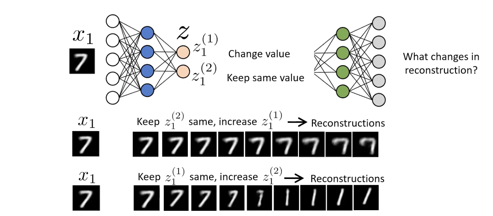
Once trained, the encoder has decided on its own what the few most important attributes of the data are. We don’t tell it “encode skin colour”; the reconstruction loss makes that the cheapest thing to encode. We can probe what was learned by visual inspection: hold one latent dimension fixed, sweep the other, decode at each step, watch what physically changes in the reconstruction.

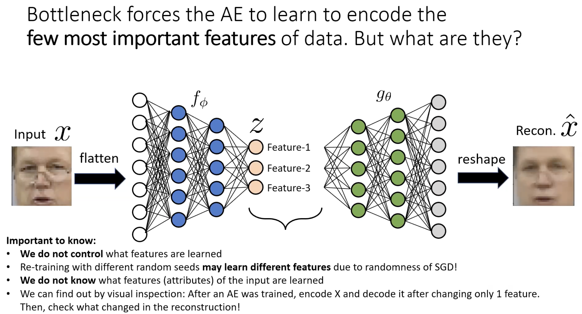
For a 2-d bottleneck on MNIST 7s, sweeping $z_1$ rotates the digit / changes curvature; sweeping $z_2$ changes stroke thickness. The network independently discovered that “angle” and “thickness” are the two most efficient features for describing a 7. That separation of factors is disentanglement, and it emerges for free.

CAUTION — Different seeds, different features

Re-training with a different random seed can yield a different set of latent features. We don’t control what the encoder learns — only the capacity it has to learn it. This makes downstream interpretation harder than supervised classification, where the output labels fix what each output means.

What autoencoders give you

1. Dimensionality reduction / compression

The bottleneck is a compressor. A streaming company example: train an AE on its movie frames, store frames as $z\in {\mathbb{R}}^{512}$ instead of $1280\times 720=921,600$ raw pixels, deploy the decoder to clients, stream codes. The compression is task-tuned (it only has to reconstruct this movie’s frames well) so it can be far smaller than a generic codec.

2. Clustering for free

Plot the latent codes of MNIST digits in ${\mathbb{R}}^2$ after training: they cluster by class even though no class label was ever shown.

The mechanism is forced by the reconstruction loss. If the encoder mapped a “0” and a “1” to the same point in $\mathcal{Z}$, the decoder would receive the same input from both and would have to produce both reconstructions from the same vector — which is impossible. So to make reconstruction unambiguous, the encoder must spread different objects apart and pull similar ones together. Clustering is a side effect of avoiding decoder ambiguity.

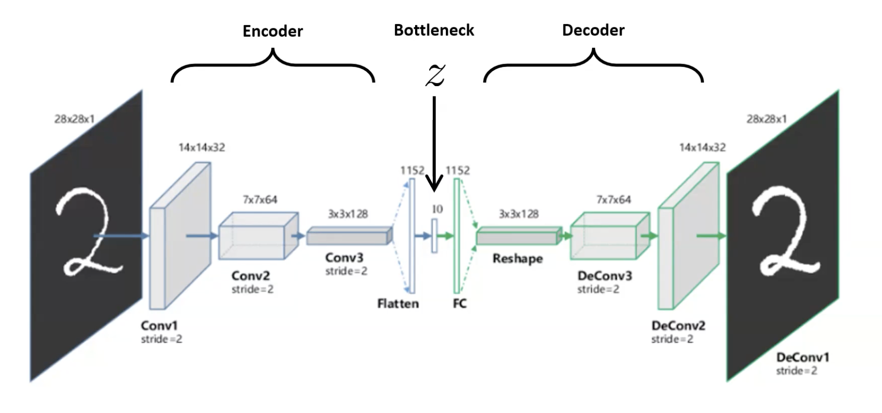
3. Convolutional autoencoders

Replace the FC encoder/decoder with conv layers (encoder) and transposed-conv / upsampling (decoder) — same idea, respects spatial structure. This is what’s used for images in practice.

4. Semi-supervised learning: pre-train then fine-tune

When labels are scarce but unlabelled data is plentiful:

1. Train an AE on the large unlabelled pile (no labels needed) — encoder learns useful features.
2. Throw away the decoder.
3. Attach a small (1–2 layer) classifier on top of the encoder.
4. Train with the small labelled set — either freeze the encoder (avoid overfitting; encoder unchanged) or fine-tune both encoder + classifier for a few SGD steps (more flexible; risks overfit).

Same recipe as transfer-learning, but the pre-training objective is reconstruction rather than ImageNet classification — useful when no large labelled source domain exists.

A friend trains an MLP autoencoder where the encoder maps ${\mathbb{R}}^{784}\to {\mathbb{R}}^{784}$ (no bottleneck). Reconstruction loss is essentially zero. They claim the encoder has learned "everything about the data." What's wrong?

The encoder has learned the identity function — $f_{\varphi }(x)=x$, $g_{\theta }(z)=z$. Zero loss is achievable trivially because the network has the capacity to just pass inputs through. No structure has been extracted; the latent code $z$ is just $x$ in a different layout, no more useful for clustering, classification, or analysis than the raw pixels. The fix is to enforce $\dim (\mathcal{Z})<\dim (\mathcal{X})$ — the bottleneck — so the encoder is forced to throw information away and decide what’s important.

Why does an autoencoder cluster MNIST digits in latent space without ever seeing a class label?

Because the encoder is graded on whether the decoder can reconstruct the input. If the encoder put a “0” and a “1” in the same place in $\mathcal{Z}$, the decoder would have no way to know which to draw — it would average them and reconstruct neither correctly, incurring a large loss for both. To minimise loss, the encoder must keep different digits at distinguishable locations. Similar inputs (all the 0s) end up close because they need similar reconstructions; different inputs end up far apart because their reconstructions diverge. Clustering is not the goal — it’s a forced consequence of unambiguous reconstruction.

Beyond reconstruction: pretext tasks

Reconstruction is not the only way to fabricate a label from the data. Pretext tasks invent a task whose answer is computable from the raw data and whose solution requires understanding image content. Examples: predict the rotation that was applied; fill in a removed patch; predict the spatial arrangement of two patches.

The pretext-task page covers Doersch et al.’s context prediction (2015): sample a centre patch and one of eight neighbours, ask the network to classify which of the 8 positions the neighbour came from. To answer correctly the network must understand “this is a cat face and that’s a cat ear, so the ear goes top-right.” A pretext-trained network’s mid-layer features (e.g. AlexNet fc6) cluster semantically — nearest-neighbour searches return cat faces near other cat faces, wheels near other wheels — without ever having seen a class label.

The Clever Hans warning

Doersch et al. discovered the network was solving the patch-position task by reading chromatic aberration — a colour-shift artefact at lens edges that gives away absolute position in the original image. The network wasn’t looking at the cat at all; it was reading the lens.

This is the Clever Hans effect (after the early-1900s horse who appeared to count but was actually reading his trainer’s micro-expressions): a model achieves high accuracy via a spurious shortcut that correlates with the label in training but doesn’t reflect the intended concept. Doersch had to specifically corrupt the colour channels to force the network to actually look at content. The lesson generalises: see clever-hans-effect for medical-imaging examples and how to defend against it.

Contrastive learning: the modern approach

Reconstruction has a flaw — the network spends capacity getting every pixel right, including irrelevant background detail. Contrastive learning sidesteps reconstruction entirely: instead of “rebuild this image,” the task is “tell same-image-pair apart from different-image-pair.”

SimCLR (Chen et al. 2020) is the canonical instantiation:

1. Sample a minibatch of $N$ images. For each $x$, apply two random augmentations $t,t^{\prime }\sim \mathcal{T}$ (crop, flip, colour jitter, blur, etc.) → two views ${\tilde{x}}_i,{\tilde{x}}_j$. Now you have $2N$ data points and $N$ positive pairs.
2. Encode each view: $h=f(\tilde{x})$ via a base encoder (typically ResNet-50). Project: $z=g(h)$ via a small MLP head.
3. Contrastive loss for a positive pair $(i,j)$: ${\ell }_{i,j}=-\log \frac{\exp (\mathrm{sim}(z_i,z_j)/\tau )}{{\sum }_{k=1}^{2N}{1}_{[k\ne i]}\exp (\mathrm{sim}(z_i,z_k)/\tau )}$ where $\mathrm{sim}(u,v)=u^{\top }v/\Vert u\Vert \Vert v\Vert$ is cosine similarity, and $\tau$ is a temperature hyperparameter.

The loss has a pull (numerator: the positive pair $z_i,z_j$ should be similar) and a push (denominator: all $2N-2$ negatives should be dissimilar). Together they shape a latent space where same-content lands close, different-content lands far apart.

The Tale of Two Representations

The phrase “latent representation” appears in both autoencoders and SimCLR — but it picks out a different vector in each. Knowing which is which matters; see latent-representation for the full disambiguation.

CAUTION — In SimCLR, $h$ is the keeper, not $z$

Autoencoders and SimCLR both produce a vector that gets called “the representation.” They are NOT the same vector.

• Autoencoder: $z$ is the bottleneck. We keep $z$ — it’s the compressed code we use for clustering / downstream tasks.
• SimCLR: $h$ comes out of the encoder $f$; $z$ comes out of the projection head $g$. After training, we throw away $g$ and keep $h$. The projection head absorbs information loss specific to the contrastive task (forgetting rotation, colour) and lets $h$ retain richer general-purpose features. When the slides say “representation,” they mean $h$. When they say “latent” they mean $z$. Don’t conflate them.

Why it works so well

SimCLR with a linear classifier on top of $h$ matches the accuracy of a fully-supervised ResNet-50 on ImageNet (76.5% top-1 with SimCLR (4×) vs ~76% supervised). This is the breakthrough result — self-supervised features can be as good as supervised ones. With only 1% of ImageNet labels, SimCLR (4×) reaches 85.8% top-5, beating heavily-engineered semi-supervised baselines.

A friend says: "If we want a good representation of an image, we should reconstruct the image — that's the only way to be sure no information was lost." Where does this reasoning go wrong, and what does SimCLR show?

Reconstruction guarantees the loss penalises every pixel error, but most pixel-level details (background texture, lighting, exact colour) are irrelevant to downstream tasks like “is this a dog?” The network spends capacity on detail it doesn’t need. Contrastive learning replaces “rebuild the image” with “tell apart same vs different objects” — which is closer to what we actually want. Two augmented views of a dog (cropped + colour-jittered + blurred) look pixel-different but share the concept “dog.” SimCLR forces the encoder to throw away the irrelevant pixel-level differences (anything an augmentation could change) and keep what’s invariant (the actual content). The result: representations as good as supervised classifiers — proving you don’t need either pixel-perfect reconstruction or class labels to learn what an image is “about.”

What ties it all together

This week is best read as variations on a single recipe:

1. Pick a target you can compute from the data alone. The input itself (AE), patch position (context prediction), augmentation-invariance (SimCLR).
2. Train a network to predict that target.
3. Throw away the prediction head; keep the encoder. The encoder’s features are the prize.
4. Use the encoder for downstream tasks — semi-supervised classification, clustering, retrieval, fine-tuning.

This umbrella is self-supervised-learning: supervised learning where the labels are fabricated from the data instead of supplied by a human. The autoencoder is the simplest example; SimCLR is the strongest known instance for vision.

Concepts introduced this week

• autoencoder — encoder-decoder trained by reconstruction; bottleneck forces compression
• representation-learning — the underlying goal: learn a vector $z$ that’s more useful for analysis than raw pixels
• self-supervised-learning — fabricate labels from the data to train without human annotation
• contrastive-learning — SimCLR; pull augmentations of the same image together, push different images apart
• pretext-task — context prediction, rotation prediction, etc. — proxy tasks that force visual understanding
• clever-hans-effect — when a model achieves high accuracy via spurious shortcuts (chromatic aberration, hospital ID, watermarks)

Connections

• Builds on u-net: autoencoders share the encoder-decoder shape but train against $x$ not $y$. Skip connections (great for U-Net) would defeat an AE — they let the input bypass the bottleneck (see week-06 problem set Q1.2).
• Builds on transfer-learning: AE pre-training + classifier fine-tuning is the same recipe as ImageNet pre-training + fine-tuning, but with a self-supervised pre-training objective rather than a supervised one. SimCLR is the modern incarnation — pre-train on unlabelled data, transfer to anything.
• Builds on data-augmentation: SimCLR turns data augmentation from a regulariser into the training signal itself. The augmentations $\mathcal{T}$ define what the encoder is told to be invariant to.
• Builds on convolutional-neural-network: the base encoder $f$ in SimCLR is a ResNet; convolutional autoencoders use the same conv layers we built in week 4 with upsampling in place of pooling for the decoder.
• Connects to overfitting: Clever Hans is overfitting to the wrong feature. The model fits the training distribution perfectly via a shortcut, then fails when the shortcut isn’t available (deployment on a new scanner, a different photographer, a clean dataset).

Open questions

• The exact role of the projection head in SimCLR is still empirical — why does throwing away $g$ and keeping $h$ give better downstream features than keeping $z$? The standard explanation (”$g$ absorbs the loss of contrastive-specific info”) is a story, not a proof.
• Variational autoencoders (VAEs) — a probabilistic version of the AE that imposes structure on $\mathcal{Z}$ — were not covered. They’re the bridge between this week and generative modelling, and they’re foundational for diffusion-style approaches. Worth picking up separately.
• Contrastive learning’s negative-sample requirement is fragile (the larger the batch, the more negatives, the better the result — SimCLR uses very large batches). Methods like BYOL claim to remove the need for negatives entirely; the why is still debated.

Problem-set lessons

The week 6 problem set is small but instructive:

• Q1 (deeper AE has worse loss): A symptom that the network is succeeding — at learning the identity function. Counter-intuitively, an AE that achieves zero reconstruction loss with no bottleneck has learned nothing useful. Lower loss is not always better when the architecture allows trivial solutions.
• Q1 (skip connections in an AE): Adding U-Net-style skips to an AE defeats the bottleneck. Information flows around the compression layer, the decoder doesn’t need a meaningful $z$, and you’re back to the identity trap with extra parameters. Skip connections are right for U-Net (where the goal is per-pixel prediction with both context and detail) but wrong for an AE (where the goal is a useful latent representation).
• Q2 (combining hospital datasets): A real-world Clever Hans setup. If hospital A is mostly negative and hospital B mostly positive, and the scanners look distinguishably different, the network will learn “scanner = label” and pass training/validation while failing at deployment. Defences: balance positive/negative within each hospital, validate on the third (balanced) hospital, normalise scanner-specific intensity / contrast, strip metadata. Same problem applies to segmentation — the artefact-based shortcut shapes the segmentation outputs the same way it shapes a classifier’s logits.