autoencoder

An autoencoder (AE) is the canonical self-supervised-learning model: input goes in, the same input is supposed to come out, and the loss penalises the difference. The architecture is two networks back-to-back — an encoder that compresses, a decoder that reconstructs. The interesting thing isn’t the reconstruction; it’s the squeezed-down latent vector $z$ in the middle. Trained well, $z$ is a high-level summary of the input, and that summary is what we use for clustering, semi-supervised classification, and compression.

Architecture

Two networks chained:

• Encoder $f_{\varphi }:\mathcal{X}\in {\mathbb{R}}^d\to \mathcal{Z}\in {\mathbb{R}}^v$ with parameters $\varphi$.
• Decoder $g_{\theta }:\mathcal{Z}\in {\mathbb{R}}^v\to \hat{\mathcal{X}}\in {\mathbb{R}}^d$ with parameters $\theta$.
• Latent code $z=f_{\varphi }(x)$ — the bottleneck output, also called the latent-representation (because it’s an internal “hidden” vector not directly observed in the input or output). In an AE this is the vector we keep: it’s the compressed encoding the network learned, and it’s the deliverable for downstream clustering / classification / retrieval.
• Reconstruction $\hat{x}=g_{\theta }(z)=g_{\theta }(f_{\varphi }(x))$.

The constraint $v<d$ is the bottleneck — the dimensionality of $z$ must be smaller than the input. Without it, the network is free to learn the identity (see below).

TIP — Why the decoder exists at all (translation/re-translation)

Think of the encoder as a translator who reads a paragraph and summarises it in three words. How do we know if those three words are a good summary? Hand them to a second translator (the decoder) and ask them to write the original paragraph back from the three words alone. If the reconstruction is faithful, the summary must have captured the important information. The decoder is not the goal — it’s the grader that gives the encoder a loss to learn from. After training, in many uses (clustering, classification head, embedding lookup), we throw the decoder away.

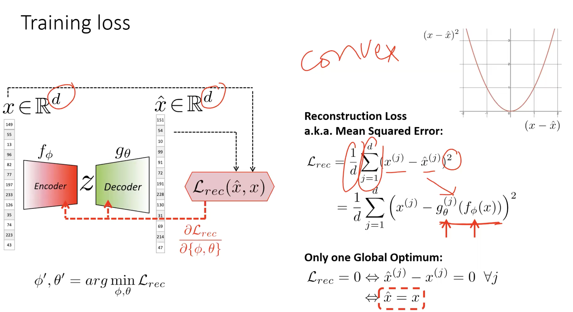
Training: reconstruction loss

Train both networks jointly to minimise mean squared error between input and reconstruction:

${\mathcal{L}}_{rec}(\hat{x},x)=\frac{1}{d}{\sum }_{j=1}^d(x^{(j)}-{\hat{x}}^{(j)}{)}^2$

The data supervises itself — the input is the target. Backprop flows from ${\mathcal{L}}_{rec}$ through the decoder, through the bottleneck, through the encoder, updating both $\varphi$ and $\theta$ jointly. No labels needed.

The global optimum is ${\mathcal{L}}_{rec}=0\iff \hat{x}=x$ — perfect reconstruction.

The trivial-solution trap

The loss is minimised when the autoencoder learns the identity function: $g_{\theta }(f_{\varphi }(x))=x$. If the bottleneck is wide enough ($v\ge d$, or even $v$ slightly less but with enough decoder capacity), the network discovers a copy-through path and reconstructs perfectly without learning anything about the data.

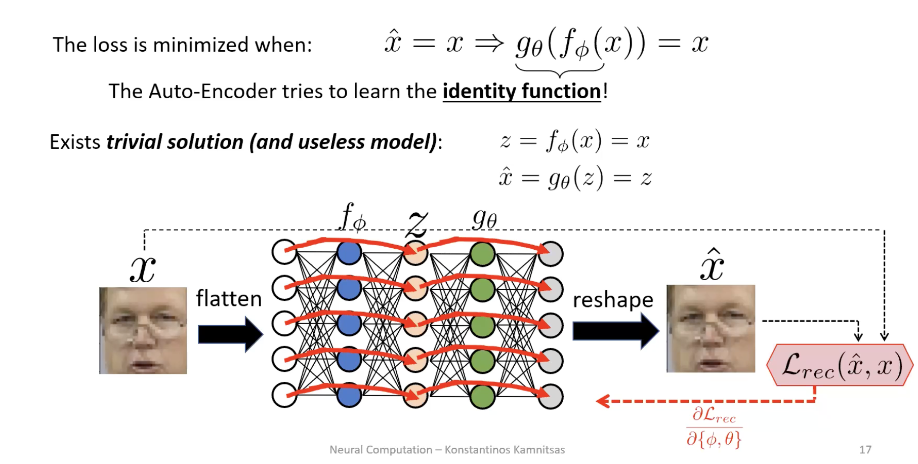
Loss is zero. Representation is useless. The latent code $z$ is just a re-encoded copy of the input, no more informative than the pixels themselves.

This is the central design constraint of an AE: make reconstruction hard enough that the network has to think.

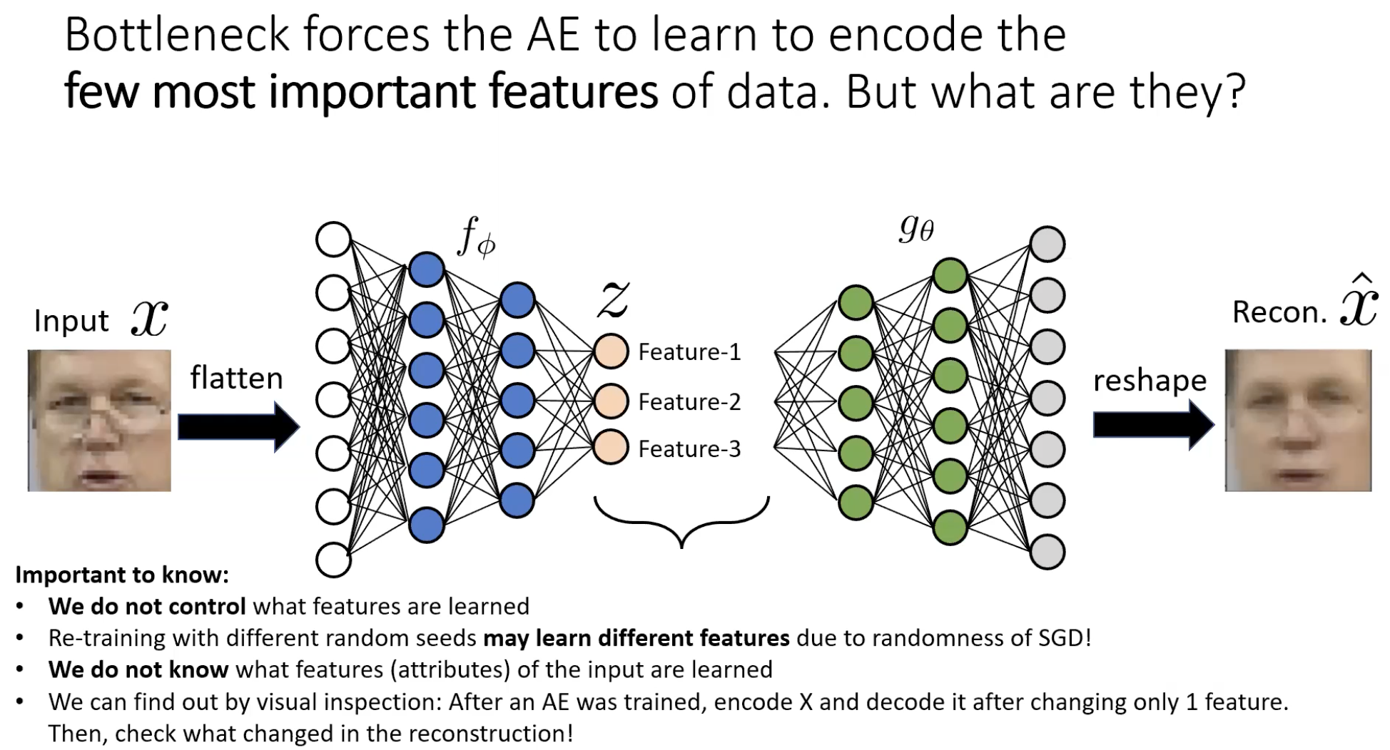
The bottleneck and what it forces

Set $v\ll d$. Now the encoder cannot preserve all the input information — it has to choose what to keep and what to throw away. Reconstruction loss penalises wrong pixel intensities, so the encoder keeps features that explain the most pixels at once:

• Skin colour — covers most of a face image. Get this wrong, thousands of pixels are off, huge MSE.
• Structural landmarks — eyes, nose, mouth: small but high-contrast, big error if displaced.
• Global shape — the silhouette / pose / digit class.

What gets thrown away:

• Glasses, eyelashes, fine textures — only a few pixels each. Cheap to lose.
• Background detail — irrelevant, smooth.

The reconstructed image is a “smoothed” version of the input — clearly the same person/digit, but blurry, with fine detail erased. That blur is the visual signature of the bottleneck doing its job.

Bottleneck width is a trade-off

Bottleneck $v$	Effect
Too narrow	Reconstruction is heavily blurred; only the most global features survive.
Sweet spot	Compact code that captures structure; reconstruction is recognisably the input minus the noise.
Too wide	Encoder learns the identity, reconstruction is near-perfect, $z$ is uninformative.

Wider/deeper networks reconstruct better; too much capacity drives the AE toward the identity. There is no universal answer — bottleneck width is a hyperparameter to tune for the downstream task.

What gets learned (and why we don’t choose)

We do not specify which features the encoder learns. The reconstruction loss + the random init + SGD jointly decide. Two consequences:

• Different random seeds → different features. Re-running training can yield qualitatively different latent codes.
• We don’t know what each $z^{(j)}$ means until we probe it. A 2-d latent code on MNIST might use $z_1$ for “thickness” and $z_2$ for “angle” — but only an experiment will tell you which.

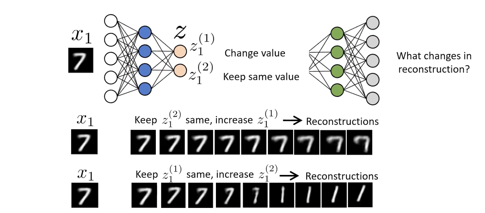
The probe is visual inspection / latent walk: hold all but one latent dimension fixed, sweep the remaining one across a range, decode at each step, look at the sequence of reconstructions to see what physically changes.

For a 2-d AE trained on MNIST 7s: sweeping $z_1$ rotates / re-curves the 7; sweeping $z_2$ thickens the stroke. The encoder discovered “angle” and “thickness” as the most efficient 2-attribute description of a 7. We did not tell it that. The clean separation of factors is disentanglement — and when an AE achieves it, it’s a happy emergent property, not a guarantee.

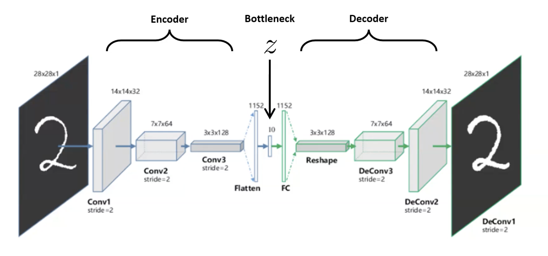
Convolutional autoencoders (CAE)

For images, replace the FC encoder/decoder with conv layers (encoder, downsampling via stride or pooling) and transposed-convs / upsampling (decoder). Same architecture pattern, but spatial structure is preserved. Standard in modern practice — flat MLP autoencoders only really show up in toy examples.

Why this works without labels — the side effects

Clustering for free

Plot the latent codes of MNIST digits in ${\mathbb{R}}^2$ after training: they cluster by class.

The encoder was never told there were digit classes. It clusters them anyway because the alternative — overlapping codes for different digits — would force the decoder to produce the same reconstruction for both, blowing up the loss. To minimise loss the encoder must keep different digits at distinguishable points in $\mathcal{Z}$. Clustering is a forced consequence of unambiguous reconstruction.

Compression / dimensionality reduction

The bottleneck is by construction a compressor — $d\to v$ values per input. For a streaming app: train an AE on the source video, store frames as $z\in {\mathbb{R}}^{512}$ instead of $\sim 10^6$ raw pixels, deploy the decoder client-side, transmit only codes. The compression is learned and task-specific — it can be tighter than a generic codec because it only has to handle frames from this distribution.

Pre-training for semi-supervised learning

When labels are scarce, but unlabelled data is abundant:

1. Pre-train. Train an AE on the (large) unlabelled pile with reconstruction loss.
2. Throw away the decoder. The encoder maps $x$ to a clustered space $\mathcal{Z}$ where the geometry is informative; that’s what we keep.
3. Attach a small classifier head $h_{\xi }:\mathcal{Z}\to \mathcal{Y}$ on top of the encoder, typically just 1–2 layers.
4. Train the head with the (small) labelled set. Two options for what to update:

	Approach 1: frozen encoder	Approach 2: fine-tune both
What’s trained	classifier head only	encoder + head jointly, often for few SGD steps
Advantage	Few parameters trained on few labels → resists overfit	Encoder gets to specialise toward the labels → potentially better representation
Disadvantage	Encoder isn’t optimised for the labelled task — may be suboptimal	All parameters are trained on few labels → easy to overfit; number of GD steps must be carefully chosen on a validation set

The encoder already knows what makes a digit a digit; the classifier just needs to learn the supervised mapping from those features to the label. Same recipe as transfer-learning but with a self-supervised pre-training objective rather than ImageNet supervision.

Common pitfalls

• Skip connections defeat AEs. Adding U-Net-style skips between encoder and decoder lets information flow around the bottleneck — perfect reconstruction, useless representation. (Week-06 problem set Q1.2.) Skip connections are right for u-net, wrong for an AE.
• Wider/deeper “improves loss” but worsens representation. A bigger network with more pooling/upsampling stages may reconstruct worse if the additional depth lets the encoder more easily hit the identity. Don’t optimise reconstruction loss as the only metric; check the downstream task.
• MSE is pixel-level. It doesn’t care about perceptual similarity — two images can be perceptually identical but differ in MSE (slight shift, slight rotation), and vice versa. For perceptual quality, swap MSE for a learned perceptual loss; for representation learning, accept that the blurriness of MSE-AE outputs is the point.

Why is "lower reconstruction loss = better autoencoder" the wrong way to think about it?

Because the loss can be driven to zero by a useless network — the identity function. An AE that achieves ${\mathcal{L}}_{rec}=0$ with $v=d$ has learned nothing about the data: every pixel passes through unchanged, $z$ is just a copy of $x$, and the supposed “representation” has no compression / no abstraction / no useful structure. The right metric is whether $z$ is useful downstream — does it cluster the data? does it work as a feature extractor for a small classifier? Reconstruction loss is a necessary signal that the encoder is preserving information, but a sufficient low loss can be achieved by cheating. Measure the downstream task.

Why does adding skip connections from encoder to decoder hurt an autoencoder, even though it helps a U-Net?

Because the goals are different. U-Net’s goal is per-pixel prediction (segmentation): it needs both deep semantic context (from the bottleneck) and high spatial precision (lost in pooling, restored by skips). The skips are essential to the task. An AE’s goal is to learn a useful $z$: the bottleneck must be the only path information can take from input to reconstruction. Skip connections create an alternative route that bypasses $z$ — the decoder can reconstruct perfectly using the skipped features alone, leaving $z$ irrelevant. Reconstruction loss → 0, representation quality → 0.

Connections

• Latent code disambiguation: see latent-representation — in an AE the kept vector is $z$ (the bottleneck); in SimCLR the kept vector is $h$ (the encoder output, before the projection head). Same word, different vector.
• Built on multi-layer-perceptron (for FC AEs) and convolutional-neural-network (for CAEs). The encoder/decoder are just standard networks; the trick is the architecture pattern and the choice of target.
• Built on u-net: same encoder-decoder shape, but trained for self-supervision instead of segmentation. Note the contrast on skip connections.
• Pre-training pattern is shared with transfer-learning — pre-train on unlabelled data, fine-tune on labels. Modern self-supervised methods like SimCLR follow the same workflow but with a stronger pre-training objective.
• Foundation for generative models — VAEs (variational autoencoders) put a probabilistic twist on this architecture, leading to controllable generation. Out of scope for this module but the natural next step.
• See representation-learning for the broader goal that AEs are one instance of.