A CNN replaces the MLP’s fully connected hidden layers with stacked convolution layers, plus pooling for downsampling. The result is a network that scales to images by sharing weights across spatial positions, while still learning a hierarchy of features end-to-end.
What a CNN looks like
A canonical CNN has three kinds of layer in roughly this order:
- Convolution layers — many filters per layer, often paired with ReLU activation. These do the feature extraction. See convolution.
- Pooling layers — periodic downsampling (typically max pooling, stride 2). See pooling.
- Fully connected (FC) layers — at the end, after flattening the spatial structure. These produce the final class scores, with softmax on the output for multi-class classification.
A typical pattern: [CONV → ReLU → CONV → ReLU → POOL] × N → FLATTEN → [FC → ReLU] × M → FC → SOFTMAX. The conv-pool block repeats times to extract increasingly abstract features at decreasing spatial resolution; the FC head turns the final feature representation into class scores.
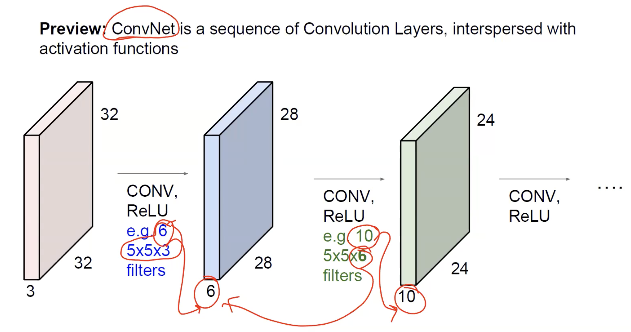
At the level of feature volumes, the picture is a chain of decreasing-spatial / increasing-depth blocks: the input () is convolved with several filters and a ReLU to give a activation map; that’s convolved with filters to give ; and so on. Spatial dimensions shrink (by valid convolution or pooling); the channel dimension grows because each layer applies many filters in parallel.
![]()
A complete CNN pipeline (here from a input) makes the alternation visible: convolution layers (Conv1 … Conv4) interleaved with subsampling/pooling layers (Sub1 … Sub3), then a fully connected head (FC5, FC6) producing the final class scores. Spatial resolution drops from → → → … → ; channel depth rises from 1 → 80 → 96 → 128 → 160. The annotations show how the kernel size shrinks deeper into the network — large kernels early to cover lots of input pixels at first, smaller kernels later because pooling has already enlarged each neuron’s receptive field.
The convolution layer
A convolution layer is the operational unit of a CNN. It wraps the convolution operation in three additional ideas:
- Multiple filters in parallel. A single filter detects one type of feature. Real layers use filters, each looking for a different pattern. Their outputs stack along the depth dimension to give a 3D output.
- Filter depth matches input depth. If the input has channels, every filter has shape . The dot product is computed across both spatial and depth dimensions, so each filter outputs a 2D map.
- Activation function applied per output. After the dot product (and a per-filter bias), an activation like ReLU. The result of the layer —
conv → activation— is called an activation map (or feature map).
For input and filters of size with stride and padding , the output volume is where the magic formula gives (and similarly for ). The depth of the output equals the number of filters, set by the layer designer.
TIP — Two depth rules to keep straight
The depth dimension causes confusion. Two rules together fix it:
- The filter’s depth is not a choice — it equals the input’s depth. If the previous layer’s output has depth , every filter in this layer has shape . The depth dimension is consumed by the per-filter dot product.
- The output’s depth is a choice — it equals the number of filters . You decide how many filters to apply; each one produces a 2D activation map; stacking them gives output depth .
So the depth pattern is: (fixed by previous layer) → (your choice this layer) → becomes the next layer’s input depth, fixing its filter depth. The number of filters is a hyperparameter at every layer; the filter depth is implied.
Counting parameters in a conv layer
Each filter has weights (one per element of the local volume) plus 1 bias. With filters:
The crucial observation: this number does not depend on or . Doubling the image size doesn’t double the parameter count of a conv layer — it just produces a larger output volume. That’s the weight-sharing payoff.
A convolution layer takes a input and applies 256 filters of size with stride 1 and padding 1. How many parameters does it have, and what's the output shape?
Each filter: parameters. Total: . Output spatial size: (same convolution preserves size). Output: .
Why multiple filters
A single filter can detect a single type of pattern — say, vertical edges. Real images contain many feature types: vertical edges, horizontal edges, diagonal edges, dots, corners, textures. A layer needs multiple filters in parallel to extract all of them.
This is the only way the network can build a rich feature representation. With one filter, the next layer sees only “where vertical edges are”. With 64 filters, it sees “where vertical edges are, where horizontal edges are, where dots are, …” — a much richer 64-channel description that subsequent layers can compose into more complex features.
ASIDE — The extreme case: convolutions
A kernel sounds useless — it has no spatial extent, just a single weight per input channel. But its depth is still the full input depth , so it performs a -dimensional dot product per spatial position. In other words: a convolution mixes information across channels at each pixel, without combining neighbouring pixels.
Concrete shape arithmetic: a input convolved with 32 filters of size gives a output. Each filter performs a 64-dimensional dot product per pixel. Spatial dimensions are unchanged; the channel count goes from 64 → 32.
This is surprisingly useful. It lets a layer change the channel count cheaply (e.g., reduce 256 channels to 64 before an expensive convolution — the “bottleneck” trick used in ResNet and Inception), and it lets the network learn channel-wise feature combinations without spatial pooling. They look trivial but are a workhorse in modern architectures.
Stacking layers: the feature hierarchy
Putting many conv layers in a row produces a hierarchy of features with two key properties:
- Increasing receptive field. Each successive layer’s neurons look at a wider patch of the original image. After many layers, a single neuron near the output can see the whole input.
- Increasing abstraction. Layer 1 detects low-level features (edges, dots) directly from pixels. Layer 2 composes those into mid-level features (corners, eyes, wheel arcs). Layer 3+ composes those into objects (faces, cars).
TIP — What "receptive field" means
The receptive field of a neuron is the patch of the original input image that influences its value. It’s an answer to “if I changed a pixel of the input, would this neuron’s value change?” — the receptive field is the set of input pixels for which the answer is yes.
- Layer 1 with kernels: each output neuron sees a patch of the input. Receptive field = 3×3.
- Layer 2 with kernels (no pooling): each layer-2 neuron sees a patch of layer-1 activations, which themselves came from patches of the input. Together, a layer-2 neuron sees a patch of the original input. Receptive field = 5×5.
- Layer 3: another step of adds 2 more on each side. Receptive field = 7×7.
Each pure conv layer with kernel size adds to the receptive field. Pooling enlarges it much faster: a pool with stride 2 doubles the receptive field of every subsequent layer (because each layer-3 neuron now sees a patch of post-pool activations, which corresponds to a patch of pre-pool activations). After several pool layers, deep neurons have receptive fields covering most or all of the input.
Why it matters: the receptive field is what the neuron “can see”. A neuron with a receptive field can detect edges; a neuron with a receptive field can detect parts of objects; a neuron whose receptive field covers the entire image can detect whole objects. The hierarchy of features is built by progressively enlarging the receptive field through depth and pooling.
This composition isn’t programmed — it emerges naturally from training on classification. Visualisations of trained CNNs consistently show:
- Early layers: edges, oriented gradients, dark spots, simple textures.
- Middle layers: eyes, ears, wheels, parts of objects.
- Late layers: faces, recognisable objects, semantic concepts.
This matches the structure of the visual cortex in animals — V1 detects edges, V4 detects parts, IT detects objects. The CNN reproduces this hierarchy spontaneously because both systems are doing the same thing: solving a hard recognition problem by composing simple detectors.
Why pooling sits between conv blocks
Three reasons to interleave pooling:
- Compute and memory. Halving spatial dimensions cuts activation count by , making deeper networks feasible.
- Shift invariance. Within each pool window, small spatial shifts are absorbed by the max operation. After several pool layers and the FC head, the final classification is largely insensitive to where in the image the object sat. See shift-invariance-equivariance.
- Larger receptive fields. Each pool layer doubles the effective receptive field of subsequent conv layers — a kernel after a pool covers a patch of the pre-pool input, and a patch of the original input after another pool. This lets later layers see the bigger picture.
There’s no rigid rule about where pools go. Some networks pool after every conv (early CNNs); some pool after every two or three convs (VGG); some skip pooling and use strided convolutions instead (ResNet).
The fully connected head
After the conv stack, the spatial feature representation has to become a class score. Two steps:
Flattening. The final feature volume is reshaped into a single vector of length . This loses spatial structure entirely (treating the whole feature volume as one long input vector to the FC layers).
Fully connected layers. One or more standard MLP-style layers, often with ReLU between them, ending in a layer with one neuron per class and softmax to produce probabilities.
The FC layers tend to dominate the parameter count in classical CNNs. In VGG16, the FC layers contain ~80% of the network’s 138M parameters even though they’re only 3 of 16 weight-bearing layers. This is the trade-off of the FC head: learnable but very parameter-heavy.
ASIDE — Replacing FC with global average pooling
Modern architectures (ResNet, EfficientNet) often use global average pooling before the final FC layer instead of flattening: average each channel of the final feature map across all spatial positions, producing a -dim vector. Then a single FC layer projects to the class scores. This drastically cuts parameters and tends to generalise better. The basic CNN we study still uses flatten + FC for clarity; just know the alternative exists.
Tensor size vs parameter count
Two different quantities people often confuse — and you’ll be asked about both in exams. They measure different things.
| Quantity | What it counts | Where it lives |
|---|---|---|
| Tensor size | How many activation values exist at a layer’s output | In memory, recomputed every forward pass |
| Parameter count | How many learnable weights the layer has | In the model file, fixed across all forward passes |
Intuitive picture: tensor size is “how many numbers come out of this layer per image”; parameter count is “how many numbers does the network remember about this layer”. Tensor size scales with input size (a bigger image produces bigger feature maps); parameter count does not (the kernel is the same size whatever image you feed it).
Counting tensor size
Tensor size = — width × height × depth of the output volume. Just multiply.
For a conv layer with input , applying filters of size with stride and padding :
(Same formula for .) For pool layers, no filter count: depth is preserved, only spatial dimensions shrink.
Counting parameters
The intuition is “count the numbers inside the kernel-block, multiply by how many kernels”:
| Layer type | Parameters | Intuition |
|---|---|---|
| Conv | One filter has weights (shape of the local volume) plus 1 bias; such filters. | |
| Pool | Pooling has no learnable weights — it’s a fixed function. | |
| FC | Every input connects to every output (weight per pair) plus one bias per output neuron. | |
| Activation (ReLU etc.) | Element-wise function, no weights. |
Notice what’s not in any of the conv-layer formulas: and . A conv layer’s parameter count doesn’t depend on the input image’s spatial dimensions — that’s the weight-sharing payoff. Only the kernel size , input depth , and number of filters matter.
For FC layers, in contrast, the parameter count does depend on input size — every input value connects to every output, so doubling the input doubles the parameters. This is why the FC head dominates parameter counts: by the time the conv stack flattens, the input vector is huge.
Worked example: a single conv layer
Take a conv layer with input , applying 16 filters of size with stride 1 and padding 2.
Tensor size: . Output: = 16{,}384 activations per image.
Parameter count: Each filter has parameters. With 16 filters: 1{,}216 parameters total.
Two very different numbers despite both being “about” this one layer. The activations grow with image size; the parameters don’t.
Worked example: a single FC layer
Take an FC layer mapping a 25{,}088-dim input vector to 4{,}096 output units (this is VGG16’s first FC layer, after flattening ).
Tensor size: Just the output dimension. Output: activations per image.
Parameter count: 103M parameters in this single layer.
Compare: VGG16’s thirteen conv layers together total ~15M parameters; this one FC layer alone is ~103M.
TIP — Why FC layers explode parameter counts
Every FC neuron has its own private weight to every input value. There’s no sharing. So when the input vector is huge (as it is right after flattening a deep feature volume), the parameter count is essentially “input size × output size” — which scales linearly in both. Conv layers escape this by reusing the same kernel everywhere; FC layers cannot, because they have no spatial structure to share over. This is why modern architectures (ResNet etc.) use global average pooling before the FC head — it collapses the spatial dimensions so the FC layer’s input is tiny.
A conv layer takes a input and applies 128 filters of with stride 1 and padding 1. Compute (a) the output tensor size and (b) the number of parameters.
(a) . Output: activations. (b) Each filter: parameters. Total: parameters. Note that the tensor is ~22× larger than the parameter count — typical for early conv layers.
An FC layer with inputs and outputs. Compute the tensor size and the parameter count.
Tensor size: (just the output dim). Parameters: — about 16.8M. The parameter count is roughly the tensor size, because every output has its own weight to every input.
Why does a conv layer's parameter count not depend on the input's spatial dimensions ?
Because the kernel is reused at every spatial position (weight sharing). The kernel itself has shape — fixed by the layer’s hyperparameters, not by how big the image is. Doubling the image size doubles the output volume (more spatial positions to apply the kernel at) but doesn’t change how many distinct weights exist in the kernel.
Two case studies
AlexNet (2012)
The breakthrough that put CNNs on the map. Won ImageNet 2012 by a huge margin (16.4% error vs the previous year’s 25.8%), kicking off the modern deep-learning era.
- Input: .
- 5 convolution layers with 96, 256, 384, 384, 256 filters (kernel sizes 11, 5, 3, 3, 3).
- 3 max-pooling layers (after conv1, conv2, conv5).
- 3 fully connected layers: 4096, 4096, 1000.
- Total: ~60M parameters.
Two things AlexNet did that we’ve already absorbed: ReLU activations everywhere (instead of sigmoid/tanh) and training on GPUs.
VGG16 (2014)
Two years later, a much deeper and more uniform design. Won ImageNet 2014 with 7.3% error.
- Input: .
- 13 convolution layers, all with padding 1.
- 5 max-pooling layers (after every block of 2-3 convs), each halving spatial size.
- Filter counts double per block: 64 → 128 → 256 → 512 → 512.
- Spatial size halves per pool: .
- 3 fully connected layers: 4096, 4096, 1000.
- Total: 138M parameters (roughly 2× AlexNet despite being deeper).
VGG’s lesson: small kernels stacked deep is more parameter-efficient than large kernels at any single layer. Two stacked convolutions cover a receptive field with fewer parameters and an extra non-linearity in between.
Walking through VGG16’s layer-by-layer parameter count
| Layer | Output shape | Parameters |
|---|---|---|
| Input | 0 | |
| conv1: 64 × 3×3 | ||
| conv2: 64 × 3×3 | ||
| pool: 2×2/2 | 0 | |
| conv3: 128 × 3×3 | ||
| conv4: 128 × 3×3 | ||
| pool: 2×2/2 | 0 | |
| … | … | … |
| pool (final) | 0 | |
| FC1 | ||
| FC2 | ||
| FC3 |
The FC1 layer alone has ~103M of the 138M total parameters — by far the biggest chunk. The 13 conv layers together account for only ~15M.
TIP — Where parameters live
Convolution layers do most of the work but have few parameters per layer (weight sharing). FC layers have many parameters per layer (no sharing). The “where do the parameters live” answer for almost any classical CNN: in the FC head. This is precisely why modern designs reduce or eliminate the FC head — it’s the highest-parameter, lowest-leverage part of the architecture.
ResNet (2016) — when stacking layers stops working
VGG showed that deeper helped, up to a point. Going much beyond ~20 layers, plain CNNs run into the degradation problem: training error gets worse as depth increases, despite the deeper network being strictly more expressive in theory. The fix is a small structural change — residual connections that add the input of each layer block back to its output. ResNet-34 (34 layers, ~21M parameters) matches or beats VGG19 (~143M parameters) on ImageNet, and the same architectural primitive scales to 50, 100, even 1000 layers. See residual-connection for the why.
Training a CNN
Same as any other neural network: forward pass to compute predictions and loss, backward pass to compute gradients, gradient descent to update weights. See backpropagation and gradient descent.
Two CNN-specific considerations:
- Backprop through convolution. A weight is used at every spatial position (weight sharing), so its gradient is the sum of contributions from every position — exactly the multivariate chain rule from week 3, applied automatically. Implementation-wise, the gradient of a convolution turns out to be another convolution (with a flipped kernel and rearranged inputs), which is why GPU-optimised convolution kernels are central to CNN training.
- Backprop through pooling. No parameters, but gradient routing matters. Max pooling routes the gradient only to the position that contained the max; average pooling spreads the gradient equally. See pooling.
CNNs aren’t only for classification
The conv layers extract a feature representation; what you do with it depends on the task.
- Classification: flatten + FC + softmax (the canonical pipeline).
- Classification + localisation: two FC heads on the feature representation — one for class scores (softmax loss), one for box coordinates (L2 loss). Add the losses.
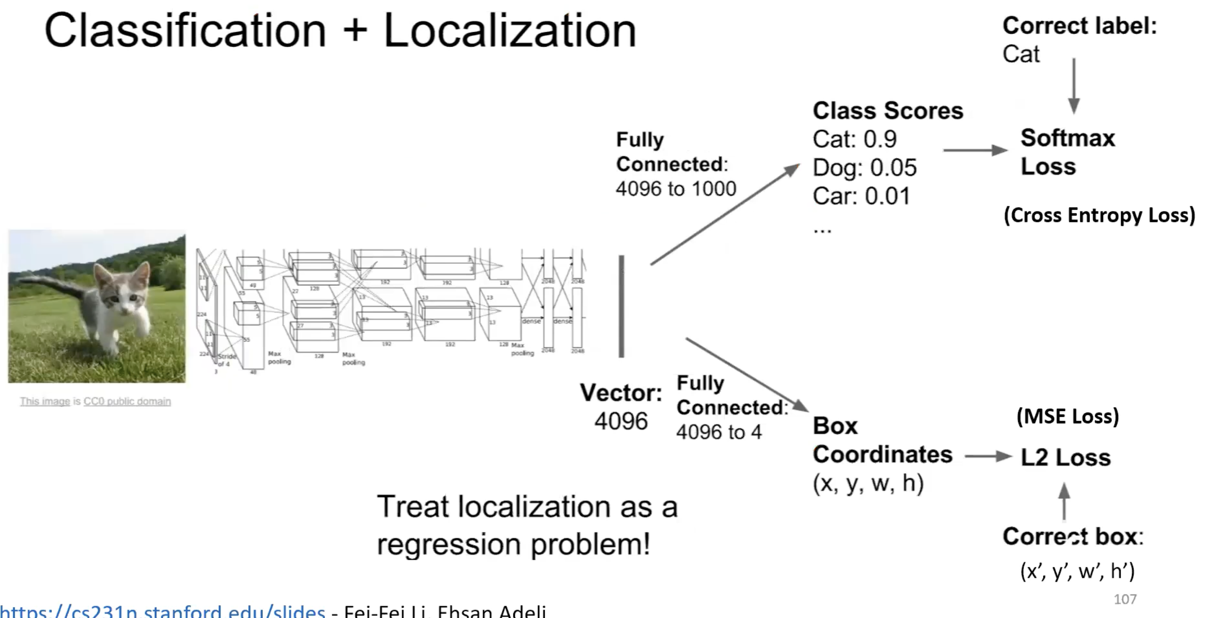
The same conv backbone produces a feature vector; one FC head predicts the class label (cat) using softmax + cross-entropy, another predicts the bounding box as a regression problem with L2 loss. Localisation is just regression dressed up — the loss is the squared distance to the ground-truth box.
- Object detection: more complex (Faster R-CNN, YOLO), but the CNN backbone is the same. See shift-invariance-equivariance for why a backbone trained for classification transfers to detection.
- Semantic segmentation: replace the FC head with more conv layers, often with upsampling, to produce a per-pixel output. Fully convolutional networks (FCNs) are the natural design; the U-Net is the canonical encoder-decoder elaboration with skip connections from encoder to decoder.
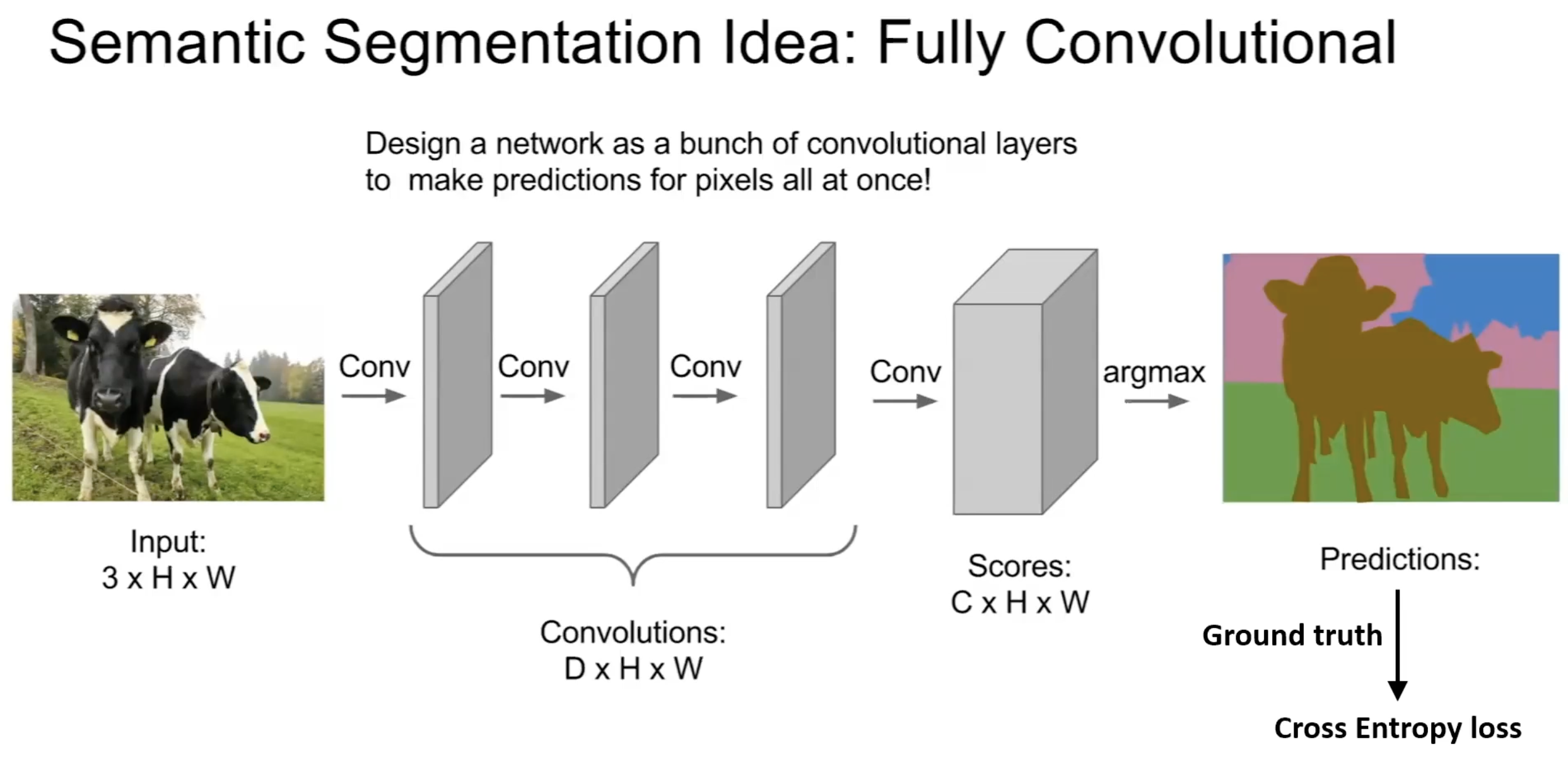
In an FCN, there are no FC layers at all — the input is convolved end-to-end into a score volume (one channel per class), and an argmax across channels gives a per-pixel class prediction. The cross-entropy loss is computed pixel-wise against a ground-truth segmentation mask. The same conv operation that classified whole images now classifies every pixel.
The CNN architecture is a feature extractor — once trained, it’s task-agnostic to a meaningful degree. This is why “CNN backbone” is a standard term: the same conv layers, with different heads, solve many vision tasks.
Related
- convolution — the operation each layer performs
- pooling — the downsampling primitive between conv blocks
- activation-functions — ReLU is the default in CNN hidden layers
- image-representation — explains why MLPs can’t replace this and why CNNs work
- shift-invariance-equivariance — symmetries that make CNNs effective for image tasks
- multi-layer-perceptron — the predecessor whose limitation on images motivated CNNs
- backpropagation — still the training mechanism; the chain rule handles weight sharing automatically
- residual-connection — the structural fix for training very deep CNNs (ResNet)
- u-net — encoder-decoder CNN architecture for segmentation
- normalization — batch normalisation is standard between CNN conv blocks
- transfer-learning — pre-trained CNN backbones as the standard starting point for new vision tasks
Active Recall
Sketch the typical layer sequence in a classification CNN, and explain the role of each layer type.
[CONV → ReLU → CONV → ReLU → POOL] × N → FLATTEN → [FC → ReLU] × M → FC → SOFTMAX. Conv layers extract features by sliding learned kernels across the input. ReLU introduces non-linearity. Pool layers downsample and add shift invariance. Flatten reshapes the spatial feature volume into a vector. FC layers mix all features into class-relevant scores. Softmax normalises into a probability distribution.
A CNN's first conv layer takes a input. The layer has 16 filters of size with padding 2 and stride 1. What's the output shape, and how many parameters does the layer have?
Output spatial size: (padding 2 makes it “same”). Output shape: . Each filter: parameters. Total: parameters.
VGG16 uses only kernels throughout. Why is this design choice better than using larger kernels?
Two stacked convolutions have the same receptive field as one convolution, but with fewer parameters per filter ( vs — and after accounting for input depth, the saving compounds). Plus, two stacks introduce two non-linearities instead of one, increasing expressiveness. Three stacked convs cover with even bigger savings. Small, deeply stacked kernels are more parameter-efficient and more expressive than large shallow ones.
Why does the convolution layer's parameter count not depend on the input image's spatial size?
Each filter has shape , regardless of or . With filters, the layer has parameters — purely a function of the layer’s hyperparameters and the input depth. The spatial dimensions only affect the output volume size, not the parameter count. This is the weight-sharing payoff: the same kernel is applied at every position, so doubling image size doesn’t double parameters.
In VGG16, almost all parameters live in just three layers (the FC layers). Why?
Conv layers share weights across all spatial positions, so they have very few parameters relative to their input size. FC layers have a unique weight per (input, output) pair: the first FC layer alone connects a flattened -dim vector to 4096 units, that’s M parameters. Conv layers throughout the network total ~15M; FC layers alone ~123M. Modern architectures often replace flatten + FC with global average pooling to slash this — VGG’s design is a snapshot of the older approach.
A friend says "convolutional networks are just MLPs with some weights forced to be equal and others forced to be zero." Is this fair?
Mostly yes — and it’s a useful conceptual framing. Forcing weights to be zero outside a small spatial neighbourhood gives the local connectivity of conv layers; forcing weights to be equal across spatial positions gives weight sharing. Both constraints reduce parameter count and bake in priors (locality and translation invariance) that suit images. So conv layers are a constrained MLP. The constraints aren’t arbitrary; they encode the inductive bias that makes CNNs efficient and effective on images.
What does "feature map" or "activation map" mean, and how is it produced?
A 2D output of one convolution filter (after applying its activation function) — one channel of the layer’s output volume. It’s produced by sliding the filter over the input volume, computing the dot product (across spatial and depth dimensions) at every position, applying the bias, then applying the activation. A layer with filters produces stacked activation maps as its output (depth ).