gaussian-kernel

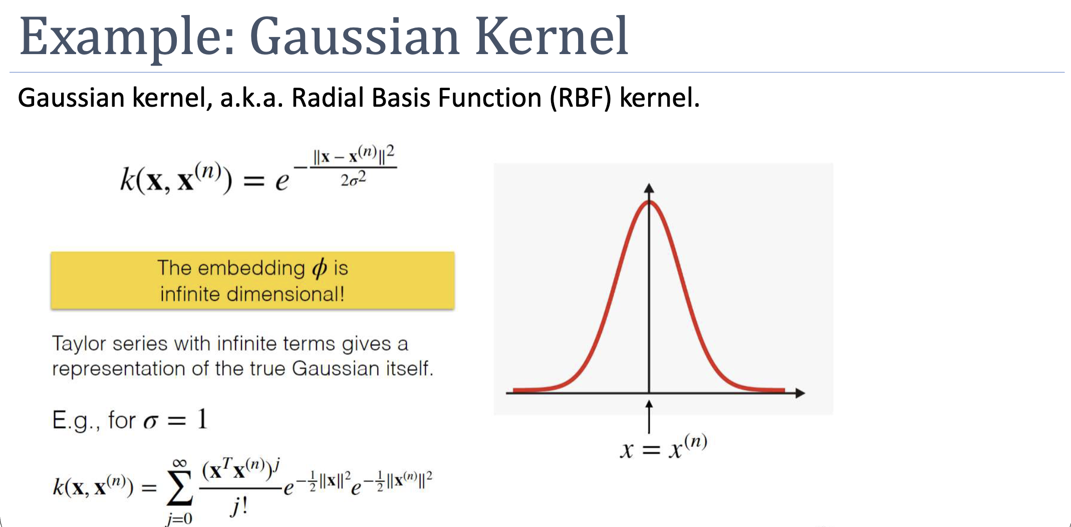
Also called the Radial Basis Function (RBF) kernel. Defined as $k(\mathbf{x},\mathbf{z})=e^{-\Vert \mathbf{x}-\mathbf{z}{\Vert }^2/2{\sigma }^2}$. The implicit feature map $\varphi$ is infinite-dimensional, so we could never compute it explicitly — but with the kernel trick we don’t have to. Its expressiveness and lack of strong assumptions make it the default kernel for non-linear SVMs.

Definition

$k(\mathbf{x},\mathbf{z})=\exp \left(-\frac{\Vert \mathbf{x}-\mathbf{z}{\Vert }^2}{2{\sigma }^2}\right)$

The output decays from $1$ (when $\mathbf{x}=\mathbf{z}$) towards $0$ (as the distance grows). The bandwidth $\sigma$ controls how quickly: small $\sigma$ → sharp peak (only very close points are similar); large $\sigma$ → broad peak (more points contribute).

Why It’s Infinite-Dimensional

Expand the kernel as a Taylor series:

$k(\mathbf{x},\mathbf{z})=e^{-\Vert \mathbf{x}{\Vert }^2/2}\cdot e^{-\Vert \mathbf{z}{\Vert }^2/2}\cdot e^{{\mathbf{x}}^{\top }\mathbf{z}}=e^{-\Vert \mathbf{x}{\Vert }^2/2}{e}^{-\Vert \mathbf{z}{\Vert }^2/2}{\sum }_{j=0}^{\infty }\frac{({\mathbf{x}}^{\top }\mathbf{z}{)}^j}{j!}$

Each term $({\mathbf{x}}^{\top }\mathbf{z}{)}^j/j!$ corresponds to a polynomial kernel of degree $j$, which has its own finite-dimensional embedding. The Gaussian kernel is an infinite weighted sum of all of them — its embedding $\varphi$ has one dimension per monomial of every degree, infinitely many. The kernel computation, of course, is just one exponential.

Validity (Sketch of Mercer Proof)

Starting from the linear kernel $k_1={\mathbf{x}}^{\top }\mathbf{z}$ (valid by inspection: $\varphi (\mathbf{x})=\mathbf{x}$), apply composition rules:

1. $k_1^j/j!$ is valid (rule: polynomial with non-negative coefficients).
2. ${\sum }_{j=0}^{\infty }{k}_1^j/j!=e^{k_1}$ is valid (rule: exponential of a kernel; or rule: sum of valid kernels).
3. Multiply by $f(\mathbf{x})f(\mathbf{z})$ with $f(\mathbf{x})=e^{-\Vert \mathbf{x}{\Vert }^2/2}$ — still valid (rule: $f\cdot k\cdot f$).

The result is exactly $k(\mathbf{x},\mathbf{z})=e^{-\Vert \mathbf{x}-\mathbf{z}{\Vert }^2/2}$ (taking $\sigma =1$ for brevity).

Practical Behaviour

• Default for non-linear SVM. Used when no domain-specific structure suggests a different kernel.
• Sensitive to $\sigma$. Too small → kernel sees only nearest neighbours, behaves like 1-NN, overfits. Too large → kernel is nearly constant, every point looks similar to every other, underfits. Cross-validate.
• Sensitive to feature scaling. Distances dominate by the largest-scale feature. Standardise inputs first.
• Universal approximator. With enough support vectors and the right $\sigma$, the Gaussian-kernel SVM can approximate any decision boundary — at the cost of greater overfitting risk.

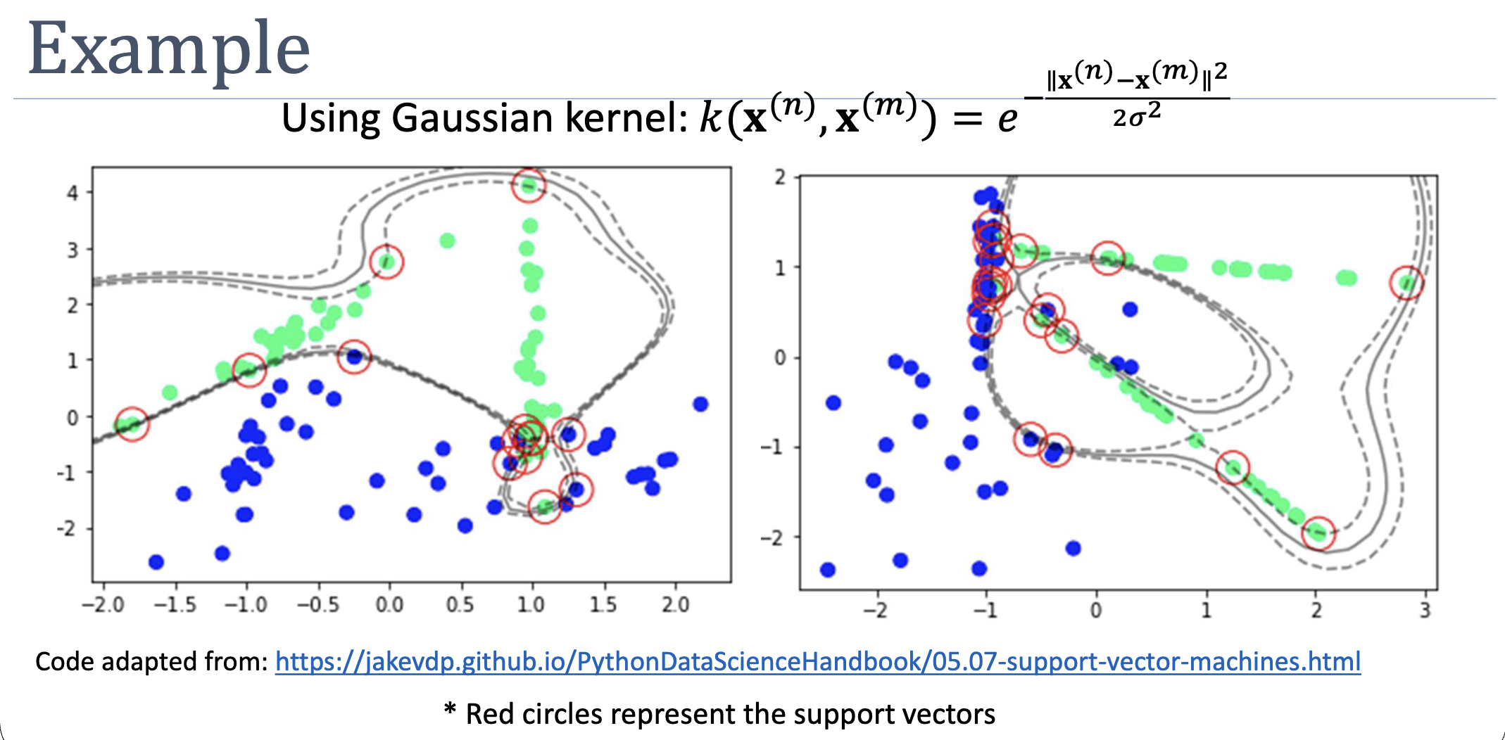
On Real Data

Two non-separable point clouds with a Gaussian-kernel SVM. The kernel produces curved, multi-modal boundaries that linear or low-degree-polynomial kernels can’t reach; support vectors (red circles) cluster near the boundary as expected.

Connection to Local Methods

The decision function $h(\mathbf{x})={\sum }_n{a}^{(n)}{y}^{(n)}{e}^{-\Vert \mathbf{x}-{\mathbf{x}}^{(n)}{\Vert }^2/2{\sigma }^2}+b$ is a weighted combination of bumps, one per support vector. In that sense, RBF SVM is structurally similar to a parametric form of kernel density classification: it asks how close the test point is to each support vector, weighted by class label and learned multiplier. Locality is built in.

Active Recall

The Gaussian kernel's embedding is infinite-dimensional, while the polynomial kernel's is finite. What does this mean in practice for the kinds of decision boundaries each can produce?

A finite-dimensional embedding restricts the boundary to a hypersurface of a fixed functional form (e.g., polynomial of degree $p$). Infinite dimensionality means the boundary can take essentially any smooth shape — bumps, ridges, isolated islands of one class, you name it. This makes Gaussian-kernel SVMs much more flexible but also more prone to overfitting; polynomial kernels constrain the hypothesis space, which acts as a built-in regulariser if the polynomial degree matches the truth.

Why does the bandwidth $\sigma$ have such a large impact on Gaussian-kernel SVM behaviour, given that we never compute the embedding?

Because $\sigma$ is the only tunable parameter inside the kernel — it directly controls how quickly similarity drops with distance. Small $\sigma$ means support vectors only “vote” near themselves, giving wiggly per-point boundaries (overfit). Large $\sigma$ means support vectors “vote” everywhere, smoothing the boundary toward something nearly linear (underfit). It plays the role analogous to polynomial degree: a single dial that traces the bias-variance frontier.

Related

• kernel-trick — what makes the infinite-dimensional embedding tractable
• mercers-condition — what licenses calling this a kernel at all
• polynomial-kernel — finite-dimensional alternative; Gaussian = infinite-degree weighted polynomial
• support-vector-machine — the canonical algorithm Gaussian kernels are paired with