kernel-trick

A “trick” because we get the benefit of working in a high-dimensional embedding $\varphi (\mathbf{x})$ — sometimes infinite-dimensional — without ever computing it. Whenever an algorithm depends on data only through inner products $\varphi (\mathbf{x}{)}^{\top }\varphi (\mathbf{z})$, we can replace those inner products with a kernel function $k(\mathbf{x},\mathbf{z})$ that returns the same value computed entirely in the original space.

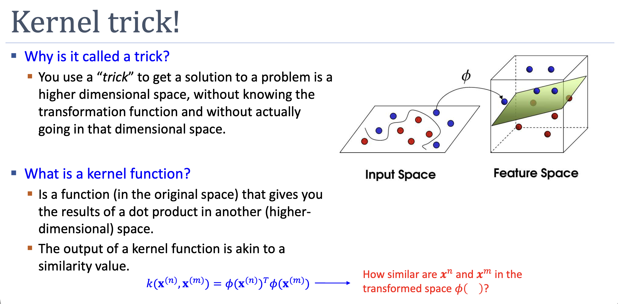
What is a Kernel Function?

A kernel function takes two points in the original input space and returns a real number:

$k:\mathcal{X}\times \mathcal{X}\to \mathbb{R},k(\mathbf{x},\mathbf{z})=\varphi (\mathbf{x}{)}^{\top }\varphi (\mathbf{z})$

It is the inner product of the two points after they’ve been mapped into some feature space $\varphi$. Conceptually, $k$ measures similarity — how aligned the two vectors are in the embedded space.

The trick: we don’t have to compute $\varphi$ to evaluate $k$. For many useful $\varphi$, there’s a closed-form expression for $k$ that uses only the original-space coordinates.

Worked Example: Polynomial Kernel of Degree 2

Take $\mathbf{x}=(x_1,x_2{)}^{\top }$ and the embedding:

$\varphi (\mathbf{x})=(1,\sqrt{2}{x}_1,\sqrt{2}{x}_2,x_1^2,x_2^2,\sqrt{2}{x}_1{x}_2{)}^{\top }$

(The $\sqrt{2}$ factors are chosen to simplify the algebra below.) Computing the inner product $\varphi (\mathbf{x}{)}^{\top }\varphi (\mathbf{z})$ explicitly:

$\varphi (\mathbf{x}{)}^{\top }\varphi (\mathbf{z})=1+2x_1{z}_1+2x_2{z}_2+x_1^2{z}_1^2+x_2^2{z}_2^2+2x_1{x}_2{z}_1{z}_2$

This factors as $(1+x_1{z}_1+x_2{z}_2{)}^2=(1+{\mathbf{x}}^{\top }\mathbf{z}{)}^2$. So:

$k(\mathbf{x},\mathbf{z})=(1+{\mathbf{x}}^{\top }\mathbf{z}{)}^2$

Two operations in the original space (one inner product, one square) replace six multiplications in the 6-dimensional feature space. As the polynomial degree grows, the saving compounds.

Why the Dual Lets Us Use Kernels

Recall the SVM dual:

$\arg {\max }_{\mathbf{a}}{\sum }_n{a}^{(n)}-\frac{1}{2}{\sum }_n{\sum }_m{a}^{(n)}{a}^{(m)}{y}^{(n)}{y}^{(m)}\varphi ({\mathbf{x}}^{(n)}{)}^{\top }\varphi ({\mathbf{x}}^{(m)})$

The data appears only through pairwise inner products $\varphi ({\mathbf{x}}^{(n)}{)}^{\top }\varphi ({\mathbf{x}}^{(m)})$. Replacing each with $k({\mathbf{x}}^{(n)},{\mathbf{x}}^{(m)})$ makes the entire optimisation independent of $\varphi$:

$\arg {\max }_{\mathbf{a}}{\sum }_n{a}^{(n)}-\frac{1}{2}{\sum }_n{\sum }_m{a}^{(n)}{a}^{(m)}{y}^{(n)}{y}^{(m)}k({\mathbf{x}}^{(n)},{\mathbf{x}}^{(m)})$

Same story for prediction:

$h(\mathbf{x})={\sum }_{n\in S}{a}^{(n)}{y}^{(n)}k(\mathbf{x},{\mathbf{x}}^{(n)})+b$

where $S$ is the set of support-vector indices. Train and predict, all without forming $\varphi$ once.

Kernel Functions Without an Explicit $\varphi$

The deeper insight: we don’t need to design $\varphi$ first. We can write down a similarity function $k(\mathbf{x},\mathbf{z})$ directly, as long as it corresponds to some valid inner product in some feature space. The condition that decides which functions qualify is Mercer’s condition (see mercers-condition).

This unlocks two things:

1. Infinite-dimensional embeddings: the RBF kernel $k(\mathbf{x},\mathbf{z})=e^{-\Vert \mathbf{x}-\mathbf{z}{\Vert }^2/2{\sigma }^2}$ corresponds to an infinite-dimensional $\varphi$, which we’d never be able to compute explicitly.
2. Non-numeric data: kernels can be defined directly on strings, trees, graphs, sets — anything for which a similarity function exists. The “feature space” $\varphi$ is implicit, never realised.

When the Kernel Trick Pays Off

In the primal, computation per training example is $O(\dim \varphi )$. In the dual with a kernel, it’s $O(\dim \mathbf{x})$ per kernel evaluation, times $N^2$ pairs. Dual is preferred when:

• $\dim \varphi \gg N$ (high-dimensional or infinite embedding, modest training set), or
• $\varphi$ is implicit (no closed form), or
• the input space is non-numeric.

When $\dim \varphi$ is small relative to $N$ (e.g., low-degree polynomial, large dataset), the primal can actually be cheaper.

Active Recall

The Gaussian kernel corresponds to an infinite-dimensional embedding. Why is this not a computational disaster?

Because we never compute the embedding. The kernel $k(\mathbf{x},\mathbf{z})=e^{-\Vert \mathbf{x}-\mathbf{z}{\Vert }^2/2{\sigma }^2}$ is evaluated entirely in the original $\mathbf{x}$-space — one subtraction, one squared norm, one exponential. The infinite dimensionality is structural (the Taylor series of $e^{{\mathbf{x}}^{\top }\mathbf{z}}$ contains arbitrarily high-order monomials), but invisible to the algorithm. We get the expressive power of an infinite feature space at the cost of evaluating a single 2-argument function.

Can any function I think captures "similarity" be used as a kernel?

No. The function must correspond to an inner product in some embedding — equivalently, the Gram matrix $K_{ij}=k({\mathbf{x}}^{(i)},{\mathbf{x}}^{(j)})$ must be symmetric and positive semidefinite for any finite set of inputs (Mercer’s condition). Otherwise the dual SVM optimisation may be ill-posed (non-convex), produce nonsense predictions, or break the geometric guarantees. In practice we either construct $k$ from validated building blocks (linear, polynomial, Gaussian) using composition rules, or verify Mercer’s condition directly.

The dual SVM's prediction is $h(\mathbf{x})={\sum }_{n\in S}{a}^{(n)}{y}^{(n)}k(\mathbf{x},{\mathbf{x}}^{(n)})+b$. Why does the prediction time depend on the number of support vectors, not the number of training examples?

Because of complementary slackness: at the optimum, $a^{(n)}=0$ for all non-support-vectors. Their contribution to the sum vanishes regardless of $k(\mathbf{x},{\mathbf{x}}^{(n)})$. Storing only the support vectors (with their $a^{(n)}$ and $y^{(n)}$) is sufficient to make any future prediction. This is a key efficiency: a typical SVM trained on $N$ points might use only $\sim \sqrt{N}$ or fewer support vectors, making prediction dramatically faster than re-evaluating against the full training set.

Related

• lagrangian — duality is what produces a kernel-friendly optimisation
• mercers-condition — when a candidate function is a valid kernel
• gaussian-kernel — most popular kernel; infinite-dimensional embedding
• polynomial-kernel — generalises the worked example above
• support-vector-machine — the canonical algorithm where the trick lives