support-vector-machine

A linear classifier that, among all hyperplanes correctly separating the training data, picks the one that sits as far as possible from the closest training point. Maximising this perpendicular distance — the margin — turns out to be a convex quadratic program with a unique global optimum.

The Idea in One Picture

Linearly separable data admits infinitely many separating hyperplanes. Some pass close to a training point on one side; some pass through the wide gap in the middle. The latter are intuitively safer: small perturbations to a point are less likely to push it across the boundary. SVMs formalise “safer” as the margin — the perpendicular distance from the boundary to the closest training point — and pick the hyperplane that maximises it.

The training points that touch the resulting margin envelope are called support vectors. They are the only points that affect the boundary; every other training point sits comfortably on its side and could be removed without changing the answer.

The Hypothesis Set

$h(\mathbf{x})={\mathbf{w}}^{\top }\mathbf{x}+b$

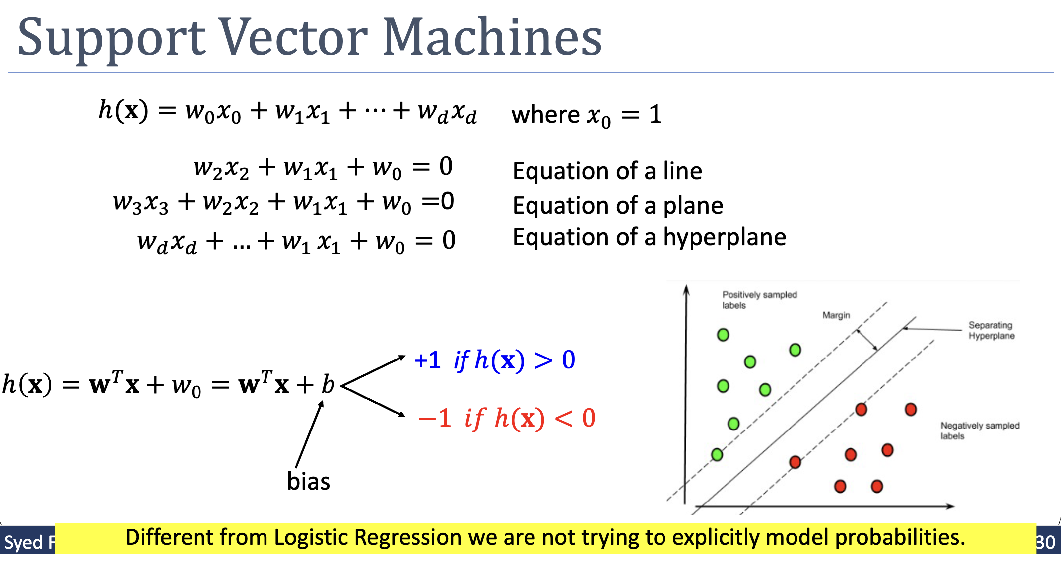
with prediction:

$\hat{y}(\mathbf{x})=\{\begin{array}{ll}+1& \text{if }h(\mathbf{x})>0\\ -1& \text{if }h(\mathbf{x})<0\end{array}$

SVM uses labels $y\in \{+1,-1\}$ rather than $\{0,1\}$ — a convention that makes the constraints cleaner. The product $y^{(n)}h({\mathbf{x}}^{(n)})$ is positive exactly when the prediction agrees with the label.

Unlike logistic-regression, SVM is not a probabilistic classifier — it doesn’t try to model $P(y\mid \mathbf{x})$. It just predicts which side of the hyperplane a point lies on.

Deriving the Optimisation

Step 1 — Express the margin. The perpendicular distance from ${\mathbf{x}}^{(n)}$ to the hyperplane $h(\mathbf{x})=0$ is $|h({\mathbf{x}}^{(n)})|/\Vert \mathbf{w}\Vert$. The margin is the minimum over training points:

$\gamma ={\min }_n\frac{|h({\mathbf{x}}^{(n)})|}{\Vert \mathbf{w}\Vert }$

Step 2 — Maximise the margin, subject to correctness. All training examples must be correctly classified — i.e., $y^{(n)}h({\mathbf{x}}^{(n)})>0$ — and among those classifiers we want the one with the largest margin:

$\arg {\max }_{\mathbf{w},b}\left\{{\min }_n\frac{y^{(n)}h({\mathbf{x}}^{(n)})}{\Vert \mathbf{w}\Vert }\right\}\text{subject to }{y}^{(n)}h({\mathbf{x}}^{(n)})>0\forall n$

The absolute value drops because, under the correctness constraint, $y^{(n)}h({\mathbf{x}}^{(n)})=|h({\mathbf{x}}^{(n)})|$.

Step 3 — Canonical rescaling. The hyperplane is unchanged if we multiply $(\mathbf{w},b)$ by any positive scalar $\kappa$. Use that freedom to fix the scale so that the closest training point satisfies $y^{(n)}h({\mathbf{x}}^{(n)})=1$. Under this rescaling:

• The constraint becomes $y^{(n)}h({\mathbf{x}}^{(n)})\ge 1$ for all $n$, with equality for at least one (the closest) point.
• The inner $\min$ in the objective becomes $1$.
• The objective collapses to maximising $1/\Vert \mathbf{w}\Vert$.

Step 4 — Convert max to min. Maximising $1/\Vert \mathbf{w}\Vert$ is equivalent to minimising $\Vert \mathbf{w}\Vert$, which is equivalent to minimising $\frac{1}{2}\Vert \mathbf{w}{\Vert }^2$. The half is conventional — it makes the gradient $\mathbf{w}$ rather than $2\mathbf{w}$. The squared norm is preferred because it’s smooth, strictly convex, and quadratic (which lets us use QP solvers).

The SVM Primal Problem

$\boxed{\arg \underset{\mathbf{w},b}{\min }\frac{1}{2}\Vert \mathbf{w}{\Vert }^2\text{subject to }{y}^{(n)}({\mathbf{w}}^{\top }{\mathbf{x}}^{(n)}+b)\ge 1\forall ({\mathbf{x}}^{(n)},y^{(n)})\in \mathcal{T}}$

This is a quadratic program: convex quadratic objective with linear inequality constraints. Properties:

• Convex. Unique global optimum; any descent method reaches it.
• Quadratic. Off-the-shelf QP solvers handle it efficiently.
• Sparse solution. At the optimum only a few constraints are active (binding with equality) — these correspond to the support vectors.

Why the Two Constraint Forms Are Equivalent

The optimal SVM solution has $y^{(n)}h({\mathbf{x}}^{(n)})=1$ for some training points (the support vectors) and $>1$ for the rest. So the constraints "$y^{(n)}h({\mathbf{x}}^{(n)})\ge 1$" and "${\min }_n{y}^{(n)}h({\mathbf{x}}^{(n)})=1$" describe the same optimum:

• The $\ge 1$ form is looser — it permits ${\min }_n>1$.
• The $=1$ form is stricter — it forces the closest point to be exactly on the margin.

Because we’re minimising $\Vert \mathbf{w}{\Vert }^2$, we want $\Vert \mathbf{w}\Vert$ to be as small as possible — i.e., the margin $1/\Vert \mathbf{w}\Vert$ to be as large as possible. The smallest $\Vert \mathbf{w}\Vert$ that satisfies $\ge 1$ everywhere is the one that achieves $=1$ at the binding constraint. The two formulations have the same optimum.

Support Vectors

At the optimum, each training point falls into one of three cases:

Condition	Meaning
$y^{(n)}h({\mathbf{x}}^{(n)})=1$	On the margin — support vector
$y^{(n)}h({\mathbf{x}}^{(n)})>1$	Strictly beyond margin — does not affect the boundary
$y^{(n)}h({\mathbf{x}}^{(n)})<0$	Misclassified — impossible in hard-margin SVM (constraint violated)

The third case can’t occur because the constraints rule it out. (For non-separable data, soft-margin SVMs introduce slack variables that allow misclassifications at a cost — covered later.)

The boundary depends only on the support vectors. Delete any non-support-vector point and re-train: the same hyperplane comes out. This is the structural reason SVMs are described as “data efficient” — only a handful of training points actually matter for the decision.

Combining With Basis Expansion

Nothing in the derivation requires that the data be linearly separable in the original space. Plug in a basis expansion $\varphi (\mathbf{x})$ and you get a non-linear SVM:

$\arg {\min }_{\mathbf{w},b}\frac{1}{2}\Vert \mathbf{w}{\Vert }^2\text{subject to }{y}^{(n)}({\mathbf{w}}^{\top }\varphi ({\mathbf{x}}^{(n)})+b)\ge 1\forall n$

The boundary is a hyperplane in $\varphi$-space, but a curved (polynomial, circular, etc.) surface in the original $\mathbf{x}$ space. With $\varphi (\mathbf{x})=(1,x_1,x_2,x_1^2,x_2^2,x_1{x}_2)$ the SVM can carve out elliptical decision boundaries — perfect for the canonical “concentric rings” example.

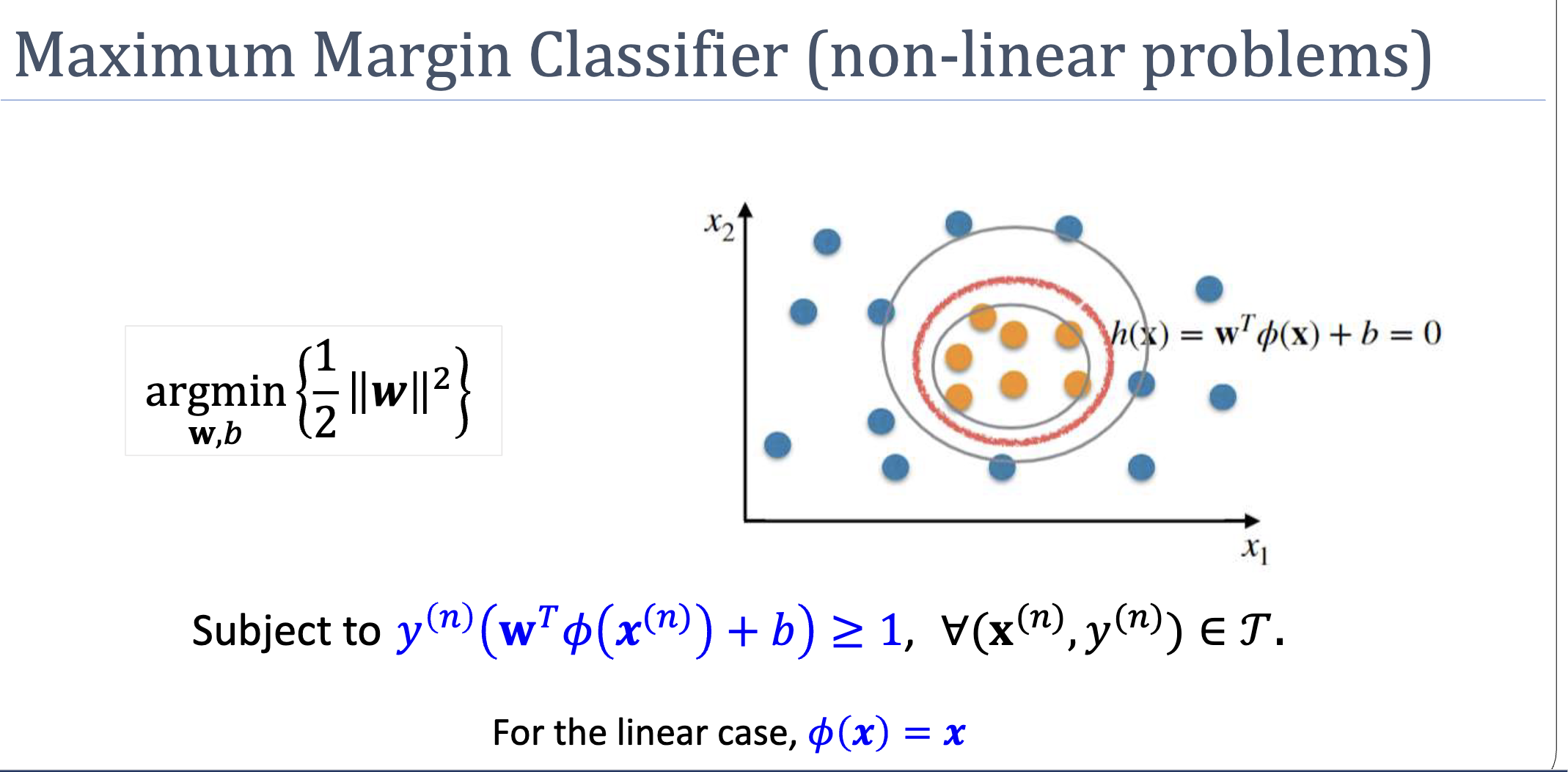
The catch: $\varphi$ may be very high-dimensional, making the QP large. The fix — using kernel functions to evaluate $\varphi (\mathbf{x}{)}^{\top }\varphi ({\mathbf{x}}^{\prime })$ without ever forming $\varphi (\mathbf{x})$ — is the kernel trick, covered in week 4 via the dual formulation (see below).

The Dual Representation

The primal QP has $\dim \varphi +1$ unknowns ($\mathbf{w},b$). Apply Lagrange duality: the constraints $1-y^{(n)}h({\mathbf{x}}^{(n)})\le 0$ each get a multiplier $a^{(n)}\ge 0$, and minimax-swap to maxmin. Setting $\partial L/\partial \mathbf{w}=0$ and $\partial L/\partial b=0$ gives:

${\mathbf{w}}^{\ast }={\sum }_n{a}^{(n)}{y}^{(n)}\varphi ({\mathbf{x}}^{(n)}),{\sum }_n{a}^{(n)}{y}^{(n)}=0$

Substituting back eliminates $\mathbf{w}$ and $b$, leaving the dual:

$\arg {\max }_{\mathbf{a}}{\sum }_n{a}^{(n)}-\frac{1}{2}{\sum }_{n,m}{a}^{(n)}{a}^{(m)}{y}^{(n)}{y}^{(m)}\varphi ({\mathbf{x}}^{(n)}{)}^{\top }\varphi ({\mathbf{x}}^{(m)})$

subject to $a^{(n)}\ge 0$ and ${\sum }_n{a}^{(n)}{y}^{(n)}=0$.

Three structural consequences:

1. The dual has $N$ unknowns, not $\dim \varphi$. When $\dim \varphi \gg N$ — high-degree polynomial expansion or Gaussian kernel — the dual is dramatically smaller.
2. Data appears only through inner products $\varphi ({\mathbf{x}}^{(n)}{)}^{\top }\varphi ({\mathbf{x}}^{(m)})$. Replace each with a kernel function $k({\mathbf{x}}^{(n)},{\mathbf{x}}^{(m)})$ evaluated in the original space — that’s the kernel-trick.
3. Sparsity from complementary slackness. KKT’s $a^{(n)}(1-y^{(n)}h({\mathbf{x}}^{(n)}))=0$ forces $a^{(n)}=0$ for every non-support-vector. The dual sum collapses to a sum over support vectors only.

Predictions in dual form:

$h(\mathbf{x})={\sum }_{n\in S}{a}^{(n)}{y}^{(n)}k(\mathbf{x},{\mathbf{x}}^{(n)})+b$

where $S$ is the support-vector index set, and $b$ is computed by averaging over support vectors:

$b=\frac{1}{|S|}{\sum }_{n\in S}\left(y^{(n)}-{\sum }_{m\in S}{a}^{(m)}{y}^{(m)}k({\mathbf{x}}^{(n)},{\mathbf{x}}^{(m)})\right)$

SVM vs Logistic Regression

	Logistic regression	SVM
Output	Calibrated probability $p_1\in (0,1)$	Class label $\pm 1$ (no probability)
Loss	Cross-entropy (smooth, all examples contribute)	Hinge / margin-based (only support vectors contribute)
Decision boundary	Any separating hyperplane the optimiser converges to	Maximum-margin hyperplane (unique)
Convex?	Yes	Yes
Handles non-separable?	Yes (still converges, weights blow up if perfectly separable)	Hard-margin SVM fails; soft-margin SVM works
Labels	$\{0,1\}$	$\{+1,-1\}$
Support for $\varphi$?	Yes (basis expansion)	Yes (and kernel trick in dual form)

For probability calibration, choose logistic regression. For maximising margin and exploiting the kernel trick, choose SVM. Both are linear-in-$\mathbf{w}$ models, both are convex, and both extend non-linearly via $\varphi$.

Related

• margin — the geometric quantity SVM maximises
• quadratic-programming — the optimisation form SVM reduces to
• non-linear-transformation — combine with SVM for non-linear boundaries
• logistic-regression — alternative linear classifier with a probabilistic output
• decision boundary — the hyperplane SVM produces
• lagrangian — duality is what produces the dual SVM and enables kernels
• kkt-conditions — complementary slackness is the structural reason SVMs are sparse
• kernel-trick — replace inner products in the dual with a kernel function

Active Recall

Why does SVM use labels $y\in \{+1,-1\}$ rather than $\{0,1\}$? Walk through the role of the product $y^{(n)}h({\mathbf{x}}^{(n)})$.

The $\pm 1$ convention makes the correct-classification check uniform: $y^{(n)}h({\mathbf{x}}^{(n)})>0$ is true exactly when the predicted side matches the true label. With $y\in \{+1\}$, $h(\mathbf{x})>0$ is needed; with $y=-1$, $h(\mathbf{x})<0$ is needed; the product handles both cases in one expression. The same trick lets us drop the absolute value $|h({\mathbf{x}}^{(n)})|$ from the margin formula under the correctness constraint, simplifying the algebra significantly.

Why does maximising the margin reduce to minimising $\Vert \mathbf{w}\Vert$ — surely larger weights should mean a larger margin?

The intuition reverses once you account for canonical rescaling. After rescaling so that the closest training point has $y^{(n)}h({\mathbf{x}}^{(n)})=1$, the perpendicular distance from that point to the boundary is $1/\Vert \mathbf{w}\Vert$. To make the margin large, $\Vert \mathbf{w}\Vert$ must be small. Geometrically, $\Vert \mathbf{w}\Vert$ controls how rapidly $h$ changes as you move away from the boundary; a steep $h$ reaches the value $1$ close to the boundary (small margin), while a gentle $h$ reaches $1$ far away (large margin). The squared norm $\frac{1}{2}\Vert \mathbf{w}{\Vert }^2$ is used in the objective because it’s smooth and yields a clean QP.

A hard-margin SVM has been trained. Suppose you receive 5 new training examples, all of which sit safely outside the margin envelope on the correct side. How does the decision boundary change?

Not at all. None of the new points become support vectors (they don’t touch the margin envelope), so the binding constraints of the QP are unchanged. The optimal $({\mathbf{w}}^{\ast },b^{\ast })$ is unchanged. This is the same property that made non-support-vectors disposable in the original training set: the boundary is determined entirely by the points sitting on the margin’s edge, regardless of how many “easy” points exist around them. (If a new point landed inside the margin or on the wrong side, the answer would be very different — for hard-margin SVM, no solution exists; for soft-margin SVM, the hyperplane shifts to accommodate it at a cost.)