Going Dual: Lagrangians, Kernels, and the Trick That Makes Them Tractable

THE CRUX: We left week 3 with an SVM that works — but it sits in a $\varphi$-space that's potentially huge (or infinite-dimensional). How do we actually solve it without paying that cost? And once we know the answer, how does it change our view of "what kind of similarity matters"?

The fix is to dualise the SVM optimisation. The primal asks for a hyperplane in $\varphi$-space; the dual reformulates this in terms of how training points relate to each other through inner products $\varphi ({\mathbf{x}}^{(n)}{)}^{\top }\varphi ({\mathbf{x}}^{(m)})$. Once it’s all about inner products, we can replace them with a kernel function $k(\mathbf{x},\mathbf{z})$ that returns the same value computed entirely in the original space — never forming $\varphi$. That’s the kernel trick. It transforms expressive but expensive embeddings into cheap function calls, opens the door to infinite-dimensional feature spaces (Gaussian kernels), and lets us define similarity directly on objects without numeric features (strings, trees, graphs).

---

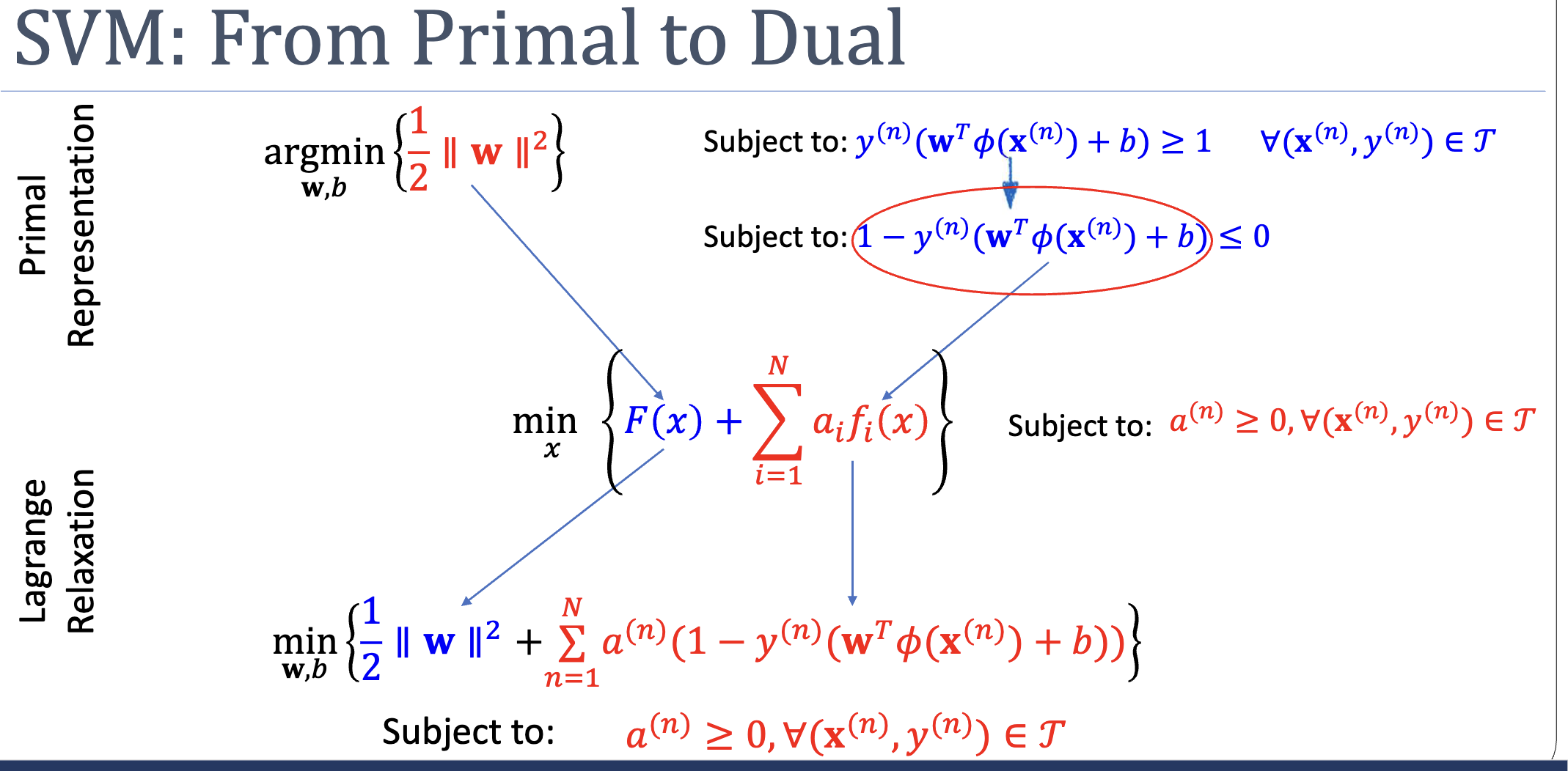
Week 3 set up the SVM primal:

$\arg {\min }_{\mathbf{w},b}\frac{1}{2}\Vert \mathbf{w}{\Vert }^2\text{subject to }{y}^{(n)}({\mathbf{w}}^{\top }\varphi ({\mathbf{x}}^{(n)})+b)\ge 1\forall n$

This is a quadratic program — convex, with a unique global optimum, solvable by off-the-shelf QP solvers. Job done, in principle. But two problems hide behind the formulation:

1. The embedding $\varphi (\mathbf{x})$ may be enormous. With 100 inputs and a degree-3 polynomial expansion, $\varphi$ has tens of thousands of components. The QP has thousands of variables. With a Gaussian-style kernel, $\varphi$ is infinite-dimensional and we can’t compute it at all.
2. The optimisation operates on the wrong currency. The primal works with the parameters $(\mathbf{w},b)$. To say anything about a new test point we still need $\varphi (\mathbf{x})$ — same cost.

This week’s payoff: a different formulation of the same problem that depends on data only through inner products $\varphi ({\mathbf{x}}^{(n)}{)}^{\top }\varphi ({\mathbf{x}}^{(m)})$. Once we have that, we can replace each inner product with a kernel function evaluated in the original space, and never touch $\varphi$ again.

Part 1: Lagrange Relaxation

The standard tool for handling inequality constraints is the Lagrangian. Instead of forbidding regions where $f_i(\mathbf{x})>0$, we fold the constraint into the objective via a non-negative multiplier $a_i\ge 0$:

$L(\mathbf{x},\mathbf{a})=F(\mathbf{x})+{\sum }_{i=1}^N{a}_i{f}_i(\mathbf{x})$

When a constraint is violated ($f_i>0$), the term $a_i{f}_i$ inflates $L$ — the optimiser is pushed away from infeasible $\mathbf{x}$. When satisfied ($f_i\le 0$), the term is non-positive and at the optimum it’s zero (the multiplier “switches off”).

But naive Lagrangian relaxation has a problem: with fixed $a_i$, the penalty might be too small to enforce the constraint. The fix is to maximise over $a_i$:

${\min }_{\mathbf{x}}{\max }_{\mathbf{a}\ge 0}L(\mathbf{x},\mathbf{a})$

If a constraint is violated, the inner max sends $a_i\to \infty$, making $L$ infinite — the outer min refuses to land there. If all constraints are satisfied, the inner max settles at $a_i=0$ (or wherever $f_i=0$), giving $L=F$. The minimax exactly reproduces the original constrained primal.

The Dual: Swapping Min and Max

The minimax requires solving a constrained max inside an unconstrained min — still awkward. The dual swaps the order:

${\max }_{\mathbf{a}\ge 0}{\min }_{\mathbf{x}}L(\mathbf{x},\mathbf{a})$

Now the inner min is unconstrained. We can attack it with ${\nabla }_{\mathbf{x}}L=0$, which often produces a closed form for ${\mathbf{x}}^{\ast }$ in terms of $\mathbf{a}$. Substituting back gives a problem purely in $\mathbf{a}$.

Two duality theorems govern when this is safe:

• Weak duality (always): ${\max }_{\mathbf{a}}{\min }_{\mathbf{x}}L\le {\min }_{\mathbf{x}}{\max }_{\mathbf{a}}L$. The dual gives a lower bound on the primal.
• Strong duality (when convex + Slater’s condition holds — both true for SVM): the inequality is equality. Dual and primal have the same optimum.

When strong duality holds, the optimum is a saddle point of $L$: a min along the $\mathbf{x}$ direction, a max along the $\mathbf{a}$ direction. Walking down-then-up or up-then-down both arrive at the same point.

KKT: When Are We Optimal?

Stationarity ($\nabla F=0$) is necessary and sufficient for unconstrained convex optimisation. With inequalities, we need more. The KKT conditions state that a primal-dual pair $({\mathbf{x}}^{\ast },{\mathbf{a}}^{\ast })$ is jointly optimal iff:

1. Stationarity. ${\nabla }_{\mathbf{x}}L=0$.
2. Complementary slackness. $a_i^{\ast }{f}_i({\mathbf{x}}^{\ast })=0$ for all $i$ — either the multiplier is zero or the constraint is active.
3. Primal feasibility. $f_i({\mathbf{x}}^{\ast })\le 0$.
4. Dual feasibility. $a_i^{\ast }\ge 0$.

Complementary slackness is the structural reason SVMs are sparse — and we’ll see why shortly.

Part 2: SVM in Dual Form

Apply this machinery to the SVM primal. First, rewrite the constraint as $f_n(\mathbf{w},b)=1-y^{(n)}({\mathbf{w}}^{\top }\varphi ({\mathbf{x}}^{(n)})+b)\le 0$. The Lagrangian:

$L(\mathbf{w},b,\mathbf{a})=\frac{1}{2}\Vert \mathbf{w}{\Vert }^2+{\sum }_{n=1}^N{a}^{(n)}(1-y^{(n)}({\mathbf{w}}^{\top }\varphi ({\mathbf{x}}^{(n)})+b)),a^{(n)}\ge 0$

The minimax is:

${\min }_{\mathbf{w},b}{\max }_{\mathbf{a}}L={\max }_{\mathbf{a}}{\min }_{\mathbf{w},b}L\text{(strong duality)}$

Take the inner min by setting partials to zero:

$\frac{\partial L}{\partial \mathbf{w}}=\mathbf{w}-{\sum }_n{a}^{(n)}{y}^{(n)}\varphi ({\mathbf{x}}^{(n)})=0\Rightarrow {\mathbf{w}}^{\ast }={\sum }_n{a}^{(n)}{y}^{(n)}\varphi ({\mathbf{x}}^{(n)})$

$\frac{\partial L}{\partial b}=-{\sum }_n{a}^{(n)}{y}^{(n)}=0\Rightarrow {\sum }_n{a}^{(n)}{y}^{(n)}=0$

Substituting ${\mathbf{w}}^{\ast }$ back into $L$ and using the second relation, $\mathbf{w}$ and $b$ both vanish from the optimisation, leaving:

$\boxed{\arg \underset{\mathbf{a}}{\max }\tilde{L}(\mathbf{a})=\sum _{n=1}^N{a}^{(n)}-\frac{1}{2}\sum _{n=1}^N\sum _{m=1}^N{a}^{(n)}{a}^{(m)}{y}^{(n)}{y}^{(m)}\varphi ({\mathbf{x}}^{(n)}{)}^{\top }\varphi ({\mathbf{x}}^{(m)})}$

subject to $a^{(n)}\ge 0$ and ${\sum }_n{a}^{(n)}{y}^{(n)}=0$.

This is the SVM dual problem. Three things to notice:

1. The unknowns are now $a^{(n)}$, not $(\mathbf{w},b)$. The dual has $N$ variables (one per training example), independent of $\dim \varphi$. When $\dim \varphi \gg N$, the dual is much smaller.
2. The data appears only through inner products $\varphi ({\mathbf{x}}^{(n)}{)}^{\top }\varphi ({\mathbf{x}}^{(m)})$. This is the opening for the kernel trick.
3. The objective is concave in $\mathbf{a}$ — still a QP, still solvable.

Sparsity from Complementary Slackness

KKT’s complementary slackness says, for each training point:

$a^{(n)}(1-y^{(n)}({\mathbf{w}}^{\top }\varphi ({\mathbf{x}}^{(n)})+b))=0$

Either:

• $a^{(n)}=0$: the point sits strictly outside the margin envelope. It contributes nothing to the dual sum — and nothing to ${\mathbf{w}}^{\ast }={\sum }_n{a}^{(n)}{y}^{(n)}\varphi ({\mathbf{x}}^{(n)})$.
• $1-y^{(n)}h({\mathbf{x}}^{(n)})=0$: the point is on the margin — a support vector. These have $a^{(n)}>0$.

So at the optimum, only support vectors have non-zero multipliers. Predictions only need the support vectors — every other training point can be deleted. Sparsity is structural, not heuristic.

Predictions in the Dual

Substituting ${\mathbf{w}}^{\ast }={\sum }_n{a}^{(n)}{y}^{(n)}\varphi ({\mathbf{x}}^{(n)})$ into $h(\mathbf{x})={\mathbf{w}}^{\top }\varphi (\mathbf{x})+b$:

$h(\mathbf{x})={\sum }_{n\in S}{a}^{(n)}{y}^{(n)}\varphi ({\mathbf{x}}^{(n)}{)}^{\top }\varphi (\mathbf{x})+b$

where $S$ is the set of support-vector indices. For $b$, use the fact that any support vector satisfies $y^{(n)}h({\mathbf{x}}^{(n)})=1$, solve for $b$, and average over all support vectors for numerical stability:

$b=\frac{1}{|S|}{\sum }_{n\in S}\left(y^{(n)}-{\sum }_{m\in S}{a}^{(m)}{y}^{(m)}\varphi ({\mathbf{x}}^{(n)}{)}^{\top }\varphi ({\mathbf{x}}^{(m)})\right)$

Predict by checking the sign of $h(\mathbf{x})$.

Notice: everything depends on $\varphi$ only through pairwise inner products.

Part 3: The Kernel Trick

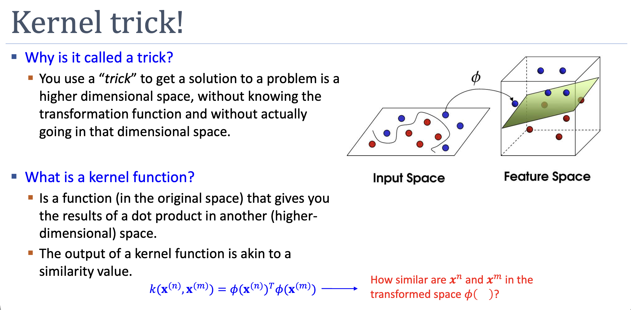
Define a kernel function $k(\mathbf{x},\mathbf{z})=\varphi (\mathbf{x}{)}^{\top }\varphi (\mathbf{z})$. Replace every inner product in the dual with $k$:

$\arg {\max }_{\mathbf{a}}{\sum }_n{a}^{(n)}-\frac{1}{2}{\sum }_{n,m}{a}^{(n)}{a}^{(m)}{y}^{(n)}{y}^{(m)}k({\mathbf{x}}^{(n)},{\mathbf{x}}^{(m)})$

$h(\mathbf{x})={\sum }_{n\in S}{a}^{(n)}{y}^{(n)}k(\mathbf{x},{\mathbf{x}}^{(n)})+b$

Now $\varphi$ is implicit. The algorithm needs only $k$, which we can often evaluate in $O(\dim \mathbf{x})$ — independent of $\dim \varphi$.

The Worked Example

Let $\varphi (\mathbf{x})=(1,\sqrt{2}{x}_1,\sqrt{2}{x}_2,x_1^2,x_2^2,\sqrt{2}{x}_1{x}_2)$ — a 6-dimensional polynomial-of-degree-2 embedding for 2D inputs. Computing the inner product:

$\varphi (\mathbf{x}{)}^{\top }\varphi (\mathbf{z})=1+2x_1{z}_1+2x_2{z}_2+x_1^2{z}_1^2+x_2^2{z}_2^2+2x_1{x}_2{z}_1{z}_2=(1+{\mathbf{x}}^{\top }\mathbf{z}{)}^2$

Six multiplications in feature space collapse into one inner product plus one square in the original space. Generalising:

$k(\mathbf{x},\mathbf{z})=(1+{\mathbf{x}}^{\top }\mathbf{z}{)}^p$

is the [[polynomial-kernel|polynomial kernel of degree $p$]] — corresponds to the embedding of all monomials of degree $\le p$. A 100-dimensional input with $p=5$ implies $\sim 10^7$ feature dimensions, but the kernel computes in 100 multiplications.

Mercer’s Condition: Which Functions Are Valid Kernels?

We’ve been assuming there’s a $\varphi$ such that $k(\mathbf{x},\mathbf{z})=\varphi (\mathbf{x}{)}^{\top }\varphi (\mathbf{z})$. Not every “similarity-shaped” function admits such a $\varphi$. The criterion is Mercer’s condition:

For any finite set of points, the Gram matrix $K_{ij}=k({\mathbf{x}}^{(i)},{\mathbf{x}}^{(j)})$ must be:

1. Symmetric: $k(\mathbf{x},\mathbf{z})=k(\mathbf{z},\mathbf{x})$.
2. Positive semidefinite: ${\mathbf{z}}^{\top }K\mathbf{z}\ge 0$ for all $\mathbf{z}$.

If both hold, $k$ corresponds to an inner product in some Hilbert space — Mercer’s theorem guarantees the existence of $\varphi$ without requiring us to compute it. Algorithmically, positive semidefiniteness keeps the SVM dual a convex QP; without it, the optimisation can wander to nonsense.

Building Kernels Without Verifying Mercer

Verifying Mercer’s condition from scratch is hard. Instead, build kernels by composition. Given valid $k_1,k_2$, the following are also valid:

$c{k}_1,f(\mathbf{x})k_{1}f(\mathbf{z}),q(k_1)\text{ for non-negative-coefficient }q,e^{k_1},k_1+k_2,k_1\cdot k_2$

The polynomial kernel is built this way: start from $k_1={\mathbf{x}}^{\top }\mathbf{z}$ (valid), apply $q(k_1)=(1+k_1{)}^p$, done.

The Gaussian (RBF) Kernel

$k(\mathbf{x},\mathbf{z})=\exp \left(-\frac{\Vert \mathbf{x}-\mathbf{z}{\Vert }^2}{2{\sigma }^2}\right)$

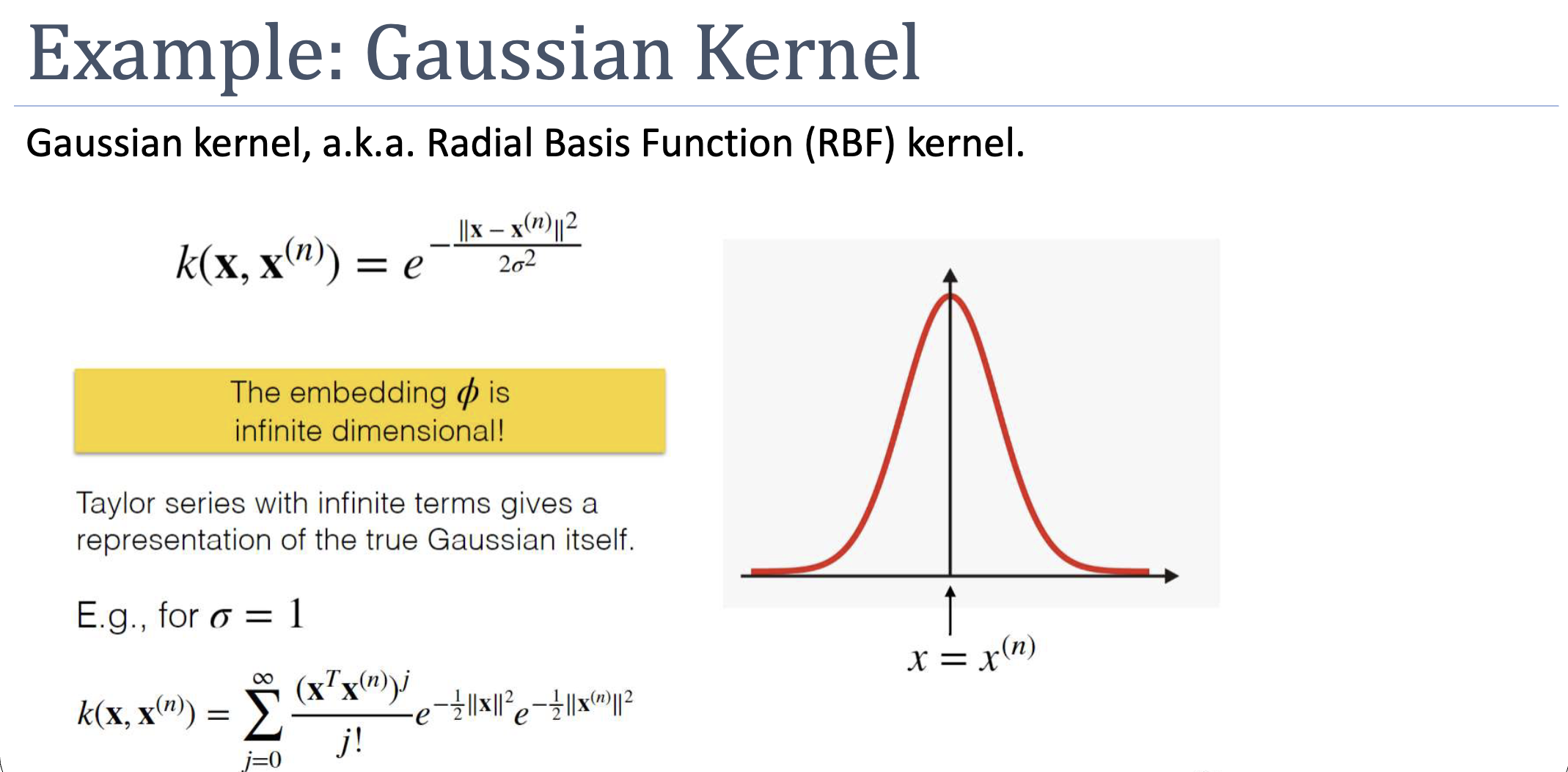
The implicit $\varphi$ is infinite-dimensional — its Taylor series contains monomials of all degrees. We could never compute $\varphi$ explicitly, but the kernel-trick sidesteps that: $k$ is one subtraction, one squared norm, one exponential.

The validity proof chains the composition rules from $k_1={\mathbf{x}}^{\top }\mathbf{z}$:

1. $k_1^j/j!$ valid (polynomial of $k_1$ with non-negative coefficients).
2. ${\sum }_j{k}_1^j/j!=e^{k_1}$ valid (sum of valid kernels, or directly the exponential rule).
3. $f(\mathbf{x})e^{k_1}f(\mathbf{z})$ with $f(\mathbf{x})=e^{-\Vert \mathbf{x}{\Vert }^2/2{\sigma }^2}$ → exactly the Gaussian kernel.

The Gaussian is the default non-linear kernel: maximally expressive, no strong structural assumptions. It pairs naturally with SVM’s margin-maximisation — even with infinite-dimensional features, maximising margin keeps the boundary regularised.

ASIDE — Kernels for non-numeric data

Once we accept that $\varphi$ doesn’t have to be constructed explicitly, kernels can be defined directly on objects without numeric features. The all-subsequence kernel for strings counts how many subsequences are shared (computable in $O(|s||t|)$ via dynamic programming). The all-subtree kernel for parse trees counts shared subtrees. The set kernel $k(A,B)=2^{|A\cap B|}$ counts shared subsets. Each of these implies an embedding $\varphi$ into a high-dimensional space — but we never realise it, just evaluate the kernel.

Part 4: When to Pick Which Kernel

Kernel	When	Caveat
Linear $k(\mathbf{x},\mathbf{z})={\mathbf{x}}^{\top }\mathbf{z}$	High-dim input, linearly separable	Can’t capture non-linearity
Polynomial $(1+{\mathbf{x}}^{\top }\mathbf{z}{)}^p$	Polynomial structure suspected (vision)	Sensitive to $p$; high-degree overfits
Gaussian / RBF	Default for non-linear; no strong prior	Needs careful $\sigma$; sensitive to feature scale
Custom (string, tree, graph)	Domain-specific structure	Must verify Mercer or compose validly

The sklearn SVC default is RBF for good reason — it’s the kernel that asks the fewest assumptions of the data.

What Could Go Wrong

• Overfitting. Gaussian kernel maps to infinite-dimensional space; without margin maximisation it would memorise the training data. Hard-margin SVM with the wrong $\sigma$ still overfits. Soft-margin SVM (next week) introduces slack to mitigate this.
• Non-Mercer kernels. A function that “looks like similarity” but fails positive semidefiniteness yields a non-convex dual, with no guarantee of finding the optimum and no margin interpretation. Stick to validated building blocks.
• Feature scaling. Both polynomial and Gaussian kernels depend on ${\mathbf{x}}^{\top }\mathbf{z}$ or $\Vert \mathbf{x}-\mathbf{z}\Vert$ — the largest-scale feature will dominate. Standardise inputs first.

---

Concepts Introduced This Week

• lagrangian — the Lagrangian function and Lagrange duality; how minimax/maxmin let us swap a constrained primal for an unconstrained-inner dual.
• kkt-conditions — Karush–Kuhn–Tucker optimality conditions for convex constrained optimisation; complementary slackness is what produces SVM’s sparsity.
• kernel-trick — replace inner products $\varphi (\mathbf{x}{)}^{\top }\varphi (\mathbf{z})$ with a kernel function $k(\mathbf{x},\mathbf{z})$ computed in the original space.
• mercers-condition — symmetric + positive-semidefinite Gram matrix tests whether a candidate function is a valid kernel.
• gaussian-kernel — Radial Basis Function kernel; infinite-dimensional embedding; default choice for non-linear SVM.
• polynomial-kernel — finite-dimensional embedding of all monomials up to degree $p$.

Connections

• Builds on week-03: takes the SVM primal (a QP in $\varphi$-space) and dualises it; the support-vector intuition becomes a structural KKT consequence rather than a mere observation.
• Builds on non-linear-transformation: kernels generalise basis expansion — same boundary shape, no need to ever materialise $\varphi$.
• Sets up later weeks: soft-margin SVM (relaxes the hard-margin constraint to handle non-separable data); regularisation and bias-variance (overfitting risk for high-capacity kernels); generalisation theory (why margin maximisation regularises infinite-dimensional embeddings).

Open Questions

• What if the data isn’t separable even in the kernel-induced space? (Soft-margin SVMs with slack variables — next week.)
• How do we choose the kernel and its hyperparameters in practice? (Cross-validation; later weeks formalise this as model selection.)
• Why does maximising margin still give a well-behaved boundary even when the implicit $\varphi$ is infinite-dimensional? (VC dimension / generalisation bounds, in weeks 8–10.)