multi-layer-perceptron

Stack multiple perceptrons in a layer, stack multiple layers one after another, feed the output of each layer into the next. That’s a multi-layer perceptron — and it’s what you need when a single straight line can’t separate your data.

Why we need more than one perceptron

A single perceptron can only draw one hyperplane — one straight line (or linear boundary) through input space. That’s fine for linearly separable classification and for data with a linear trend, but it fails on anything curvier. The XOR pattern, or any dataset with positive examples on opposite corners, simply cannot be split by a single line.

The fix: use multiple perceptrons. Two perceptrons in a first layer each draw their own boundary, carving space into regions. A perceptron in the next layer combines their outputs to produce a more complex decision surface. Stack enough of these and you can approximate any reasonable function — that’s the power of an MLP.

MLPs are also called feed-forward neural networks — “feed-forward” because information flows only in one direction, from input to output, never backward during inference. (Training is a different story — see backpropagation.)

TIP — Layers as a hierarchy of abstraction

The deep idea behind layered networks isn’t really “more capacity”; it’s compositional learning. Each layer solves a simpler sub-problem, and stacking layers builds up to solve a complex one.

Think of building a house. You can’t go directly from atoms to a finished house. But you can go atoms → materials (wood, metal, glass) → components (walls, beams, windows) → rooms → house. Each step is a manageable transformation; the complexity emerges from the composition.

Or think of how you learned to read: letters → words → grammar → meaning. You don’t memorise every possible sentence — you build up layers of understanding.

A neural network does the same thing automatically. Early layers learn simple features (edges, textures); middle layers compose those into parts (shapes, motifs); later layers compose parts into concepts (objects, classes). Each layer breaks the problem into something the next layer can build on. This is what makes deep networks dramatically more powerful than shallow ones, even when they have the same total parameter count.

Anatomy of an MLP

An MLP consists of:

• Input layer — just the features; no computation happens here, it’s a placeholder for $\mathbf{x}$. Width is fixed by your data: if your input has $D$ features, the input layer has $D$ “nodes”.
• Hidden layers — one or more layers of perceptrons between input and output. “Hidden” because they’re not directly observable from outside; they process intermediate representations. Width is a free design choice — pick 3, 30, or 3000 neurons, the math doesn’t care.
• Output layer — the final layer. Width is fixed by your task: 1 unit for binary classification / regression, $k$ units for $k$-class classification.

In a fully connected MLP, every neuron in layer $\ell$ is connected to every neuron in layer $\ell -1$. This is the default architecture; other connection patterns (e.g. convolutional, recurrent) come later in the module.

Each individual hidden/output neuron is a soft perceptron — a perceptron with a smooth activation like the sigmoid function (not sign, because gradient descent needs differentiability).

What determines each layer’s width vs. each neuron’s weight count

A common confusion: “is the number of neurons in a layer tied to the number of features?” No — the layer-width question and the per-neuron-weight-count question have different answers:

Question	Answer
How many neurons in a hidden layer?	A free design choice (a hyperparameter). Pick whatever you want.
How many weights does each neuron in layer $\ell$ have?	Exactly the width of layer $\ell -1$ — one weight per incoming connection.

So a chef in layer $\ell$ has as many entries in their recipe as there are ingredients on the counter — which equals the previous layer’s width. The number of chefs in the kitchen is independent: you can hire 3 or 300, they all read the same counter.

CAUTION — Features don't "own" weights; (neuron, feature) pairs do

It is tempting to read $W^{\ell }$ as “each feature has a list of weights”. The cleaner picture is that each weight $w_{j,k}^{\ell }$ belongs to a (neuron $j$, feature $k$) pair. Rows of $W^{\ell }$ are chef recipes (one weight per feature); columns are “how every chef cares about feature $k$“. The standard mental model is rows-as-recipes — that’s the picture that generalises cleanly into matrix multiplication and into backprop.

Notation (this is important)

The notation the module uses is worth memorising — it appears in exam questions and in every subsequent week.

Symbol	Meaning
$L$	Total number of layers (superscript $1$ = input layer, $L$ = output layer)
$m$	Width of a layer (number of neurons); can vary between layers
$a_j^{\ell }$	Activation of neuron $j$ in layer $\ell$ — the output after the activation function
$z_j^{\ell }$	Weighted input to neuron $j$ in layer $\ell$ — the raw pre-activation value
$w_{jk}^{\ell }$	Weight from neuron $k$ in layer $\ell -1$ to neuron $j$ in layer $\ell$. Superscript = destination layer; subscript = (destination unit, source unit).
$b_j^{\ell }$	Bias of neuron $j$ in layer $\ell$

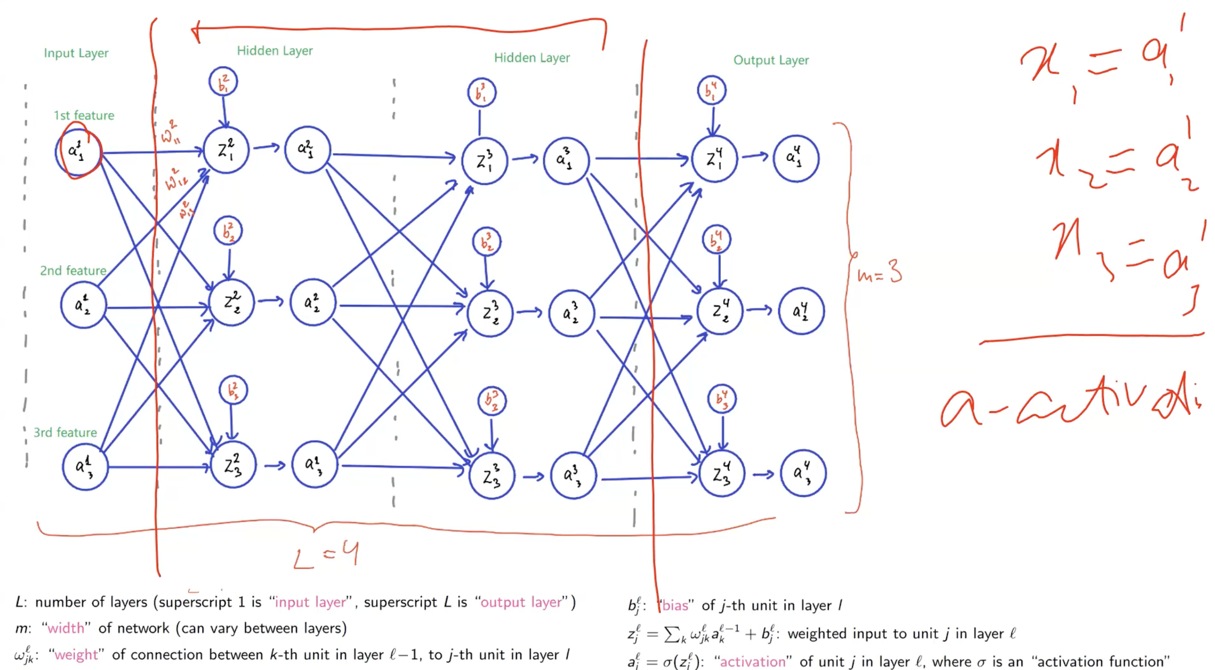
The core equations for a single neuron in layer $\ell$:

$z_j^{\ell }={\sum }_k{w}_{jk}^{\ell }{a}_k^{\ell -1}+b_j^{\ell }$ $a_j^{\ell }=\sigma (z_j^{\ell })$

where $\sigma$ is an activation function (sigmoid, ReLU, tanh, …). The input layer uses $a_k^1=x_k$ directly — there is no weighted sum or activation at layer 1.

Each neuron in a layer has its own weights

A common point of confusion: “if every neuron in layer $\ell$ reads the same activations $a_k^{\ell -1}$ from the previous layer, don’t they all compute the same $z$?”

No — because each neuron has its own private weight vector and bias. The subscript $j$ on $w_{jk}^{\ell }$ and $b_j^{\ell }$ is doing the work: it labels which neuron the weight belongs to.

Intuition: a kitchen of chefs

Picture a hidden layer as a kitchen with $m$ chefs. The previous layer dumps a tray of ingredients onto a shared counter — flour, sugar, butter, eggs (these are the activations $a_1^{\ell -1},a_2^{\ell -1},a_3^{\ell -1},a_4^{\ell -1}$). Every chef has access to the same tray. That part is true.

What makes the chefs different is their recipes. A recipe tells a chef how much of each ingredient to use — those amounts are the weights $w_{j,k}^{\ell }$ — plus a “house seasoning” they always add, which is the bias $b_j^{\ell }$.

Chef $j$	Flour	Sugar	Butter	Eggs	Bias	Output $z_j^{\ell }$
1	2	1	0.5	3	+salt	Cake batter
2	1	0	2	1	+pepper	Pastry dough
3	0.1	4	0	0	+cinnamon	Caramel

All three chefs perform the same kind of operation — weigh out some of each ingredient, add their house seasoning, mix. But because the amounts differ wildly per recipe, they end up with three completely different dishes.

The activation $\sigma$ is the oven: each chef sticks their mixture in to bake, applying a non-linear transformation (browning, rising, hardening). The output $a_j^{\ell }=\sigma (z_j^{\ell })$ that goes to the next layer is the baked dish, not the raw mixture.

So “they’re all just doing a linear combination of the same inputs” is true the way “they’re all just combining flour, sugar, butter, eggs” is true — but the amounts are different per chef, which is why you get cake, pastry, and caramel from one shared tray.

Matrix form: the kitchen’s recipe book

Stack every chef’s recipe as one row of a matrix and the whole layer becomes a single equation:

${\mathbf{z}}^{\ell }=W^{\ell }{\mathbf{a}}^{\ell -1}+{\mathbf{b}}^{\ell }$

For the kitchen above:

$W^{\ell }=\left(\begin{array}{c}\text{Chef 1’s recipe}\\ \text{Chef 2’s recipe}\\ \text{Chef 3’s recipe}\end{array}\right)=\left(\begin{array}{cccc}2& 1& 0.5& 3\\ 1& 0& 2& 1\\ 0.1& 4& 0& 0\end{array}\right)$

$W^{\ell }$ has shape (neurons in layer $\ell$) × (neurons in layer $\ell -1$). Each row is one chef’s recipe. The matrix-vector product is just “for each chef, calculate their dish from the ingredients on the counter” — one $z_j^{\ell }$ per row.

What the next layer does

Cake, pastry, and caramel become the new ingredients on the counter for layer 2. Layer 2’s chefs each have their own recipe for combining those intermediate dishes — a wedding cake, a danish, a praline tart. Same picture one level up. This is why depth helps: each layer turns dishes from the previous layer into more complex compositions, building from raw flour all the way up to the final output.

CAUTION — Initialise to break symmetry

If every chef were handed the same recipe at the start (all weights initialised to zero or the same value), they’d all bake identical dishes. The same gradient update would land on every chef equally, so they’d stay clones forever — the layer would collapse to a single effective neuron regardless of width. This is exactly why weight-initialization samples weights from a random distribution: to give every chef a different starting recipe so they specialise into distinct dishes from step zero.

TIP — Why use $a$ instead of $x$ for activations

At the input layer, the “activations” are just the raw features, so it looks odd to not call them $x$. But layers 2 onwards receive activations from the previous layer — not raw inputs — and using $a$ uniformly across all layers makes the recurrence clean: $a_j^{\ell }$ depends on $a_k^{\ell -1}$, regardless of which layer you’re in. A single piece of notation covers every layer.

Why activations must be non-linear

Stacking layers without non-linearity buys you nothing. Suppose every neuron just computed $z^{\ell }=W^{\ell }{a}^{\ell -1}+b^{\ell }$ — no $\sigma$. Compose two layers:

$a^3=W^3{a}^2+b^3=W^3(W^2{a}^1+b^2)+b^3=(W^3{W}^2)a^1+(W^3{b}^2+b^3)$

That’s just one linear transformation with combined weights $W^3{W}^2$ and combined bias $W^3{b}^2+b^3$. No matter how many layers you stack, a network of pure linear layers is mathematically equivalent to a single linear layer — same expressive power as a single perceptron, completely defeating the point of having multiple layers.

The non-linear activation function (sigmoid, tanh, ReLU) is what breaks this collapse. With a non-linearity between layers, $a^3=\sigma (W^3\sigma (W^2{a}^1+b^2)+b^3)$ does not simplify to a single linear transformation. Each layer can now genuinely transform the representation in ways the previous layer couldn’t, and the composition is genuinely richer than any single layer.

So the activation function isn’t just a differentiability fix (see sigmoid function) — it’s also what makes multi-layer networks more powerful than single-layer ones in the first place. Without it, depth is wasted.

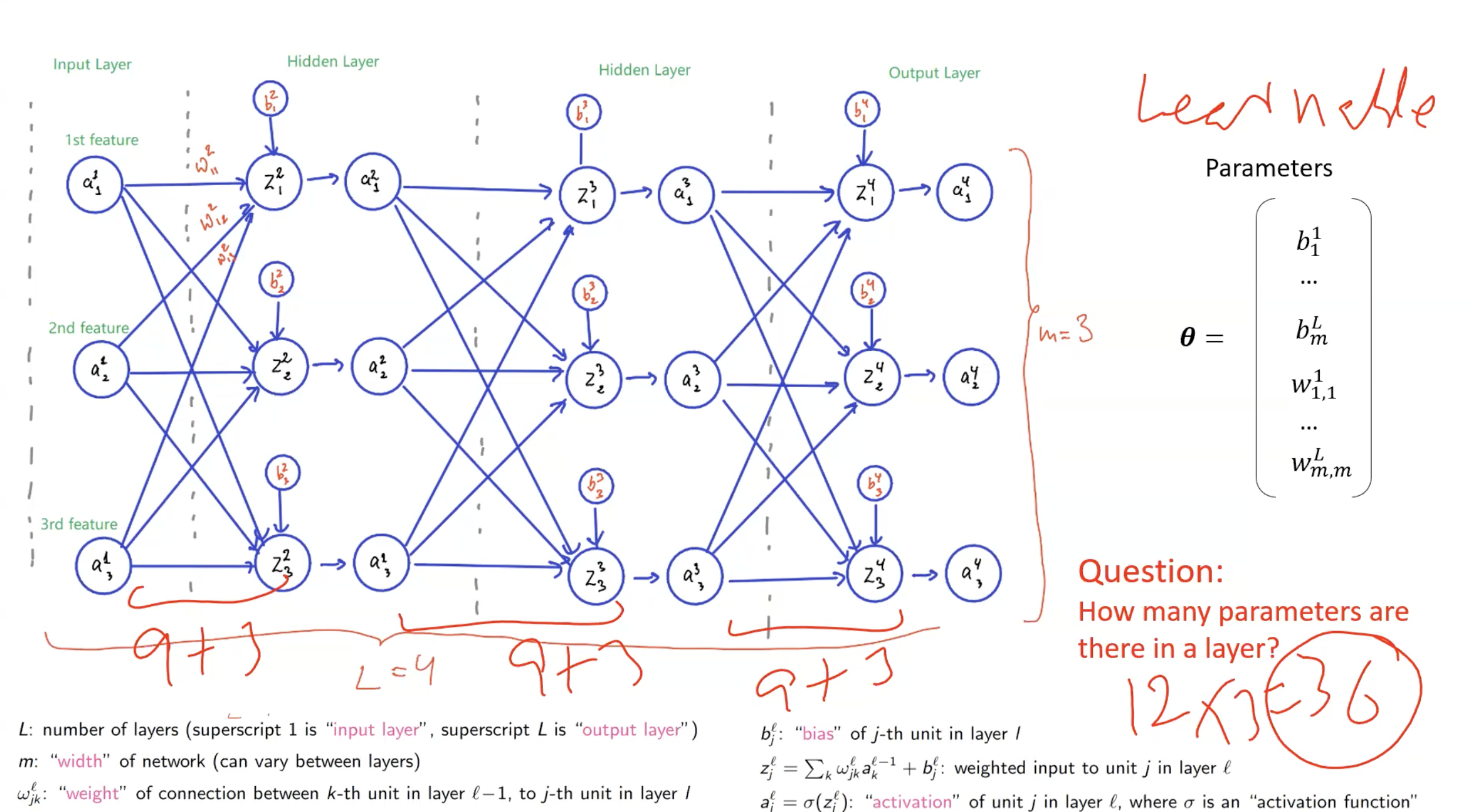
Counting parameters

Exam questions routinely ask you to count parameters. The recipe:

For layer $\ell$ with $m_{\ell }$ neurons, receiving input from a layer with $m_{\ell -1}$ neurons:

• Weights: $m_{\ell }\times m_{\ell -1}$ (one per connection, fully connected)
• Biases: $m_{\ell }$ (one per neuron in layer $\ell$)
• Total parameters for layer $\ell$: $m_{\ell }\times (m_{\ell -1}+1)$

For the whole network: sum over all layers $\ell =2,\dots ,L$. The input layer contributes no parameters.

Worked example

For the network shown in the lecture (input: 3 features, three hidden/output layers of 3 neurons each, so $L=4$, each layer width 3):

• Layer 1 → Layer 2: $3\times 3+3=12$ parameters
• Layer 2 → Layer 3: $3\times 3+3=12$ parameters
• Layer 3 → Layer 4: $3\times 3+3=12$ parameters
• Total: 36 parameters.

(Note: the number of activations — the $a_j^{\ell }$ values — are not learnable parameters. Only weights and biases are.)

Worked example: forward pass through a 2-hidden-layer MLP

To pin down what each chef does mechanically, let’s trace one input all the way through a small network. Architecture:

• Input layer ($\ell =1$): 3 features
• Hidden layer 1 ($\ell =2$): 3 neurons, ReLU
• Hidden layer 2 ($\ell =3$): 2 neurons, ReLU
• Output layer ($\ell =4$): 1 neuron, sigmoid (binary classification)

ReLU here means $\sigma (z)=\max (0,z)$ — “if a chef’s mixture comes out negative, the oven discards it and produces 0; otherwise it bakes it as-is.”

Input

${\mathbf{a}}^1=\mathbf{x}=\left(\begin{array}{c}1\\ 2\\ -1\end{array}\right)$

Three ingredients on the counter for layer 2’s chefs to use.

Hidden layer 1 (3 chefs)

The recipe book — each row is one chef’s recipe; each column is one ingredient:

$W^2=\left(\begin{array}{ccc}0.5& 1.0& -0.5\\ -2.0& 0.5& 1.0\\ -0.2& 1.5& 0.5\end{array}\right),{\mathbf{b}}^2=\left(\begin{array}{c}0.1\\ 0.0\\ 0.3\end{array}\right)$

The three chefs have completely different recipes:

• Chef 1 $(0.5,1.0,-0.5)$ — likes ingredient 2, mildly likes 1, dislikes 3.
• Chef 2 $(-2.0,0.5,1.0)$ — hates ingredient 1, mild on 2, likes 3.
• Chef 3 $(-0.2,1.5,0.5)$ — ingredient-2-obsessed.

Compute each chef’s pre-activation $z_j^2={\sum }_k{w}_{j,k}^2{a}_k^1+b_j^2$:

z^2_1 &= 0.5(1) + 1.0(2) + (-0.5)(-1) + 0.1 = 3.1 \\ z^2_2 &= (-2.0)(1) + 0.5(2) + 1.0(-1) + 0.0 = -2.0 \\ z^2_3 &= (-0.2)(1) + 1.5(2) + 0.5(-1) + 0.3 = 2.6 \end{aligned}$$ Or, in one matrix equation: $$\mathbf{z}^2 = W^2 \mathbf{a}^1 + \mathbf{b}^2 = \begin{pmatrix} 3.1 \\ -2.0 \\ 2.6 \end{pmatrix}$$ Apply ReLU per chef: $$\mathbf{a}^2 = \text{ReLU}(\mathbf{z}^2) = \begin{pmatrix} 3.1 \\ 0 \\ 2.6 \end{pmatrix}$$ Chef 2's mixture came out negative — the oven discarded it. Downstream layers will see "Chef 2 had nothing to contribute today". ### Hidden layer 2 (2 chefs) **This is the key shift.** Layer 3's chefs do *not* see the original $\mathbf{x}$. Their counter has been re-stocked with the **outputs of layer 2** — Chef 1's dish (3.1), Chef 2's nothing (0), and Chef 3's dish (2.6) are the new ingredients. $$\mathbf{a}^2 = \begin{pmatrix} 3.1 \\ 0 \\ 2.6 \end{pmatrix} \quad \leftarrow \text{ingredients for layer 3}$$ Layer 3's recipe book has 2 rows (2 chefs) and 3 columns (3 incoming ingredients): $$W^3 = \begin{pmatrix} 0.4 & -1.0 & 0.6 \\ 1.0 & 0.5 & -0.3 \end{pmatrix}, \qquad \mathbf{b}^3 = \begin{pmatrix} -0.5 \\ 0.2 \end{pmatrix}$$ $$\begin{aligned} z^3_1 &= 0.4(3.1) + (-1.0)(0) + 0.6(2.6) + (-0.5) = 2.30 \\ z^3_2 &= 1.0(3.1) + 0.5(0) + (-0.3)(2.6) + 0.2 = 2.52 \end{aligned}$$ Both positive, so ReLU passes them through: $$\mathbf{a}^3 = \begin{pmatrix} 2.30 \\ 2.52 \end{pmatrix}$$ ### Output layer (1 chef) The final chef's ingredients are the two layer-3 outputs: $$W^4 = \begin{pmatrix} 0.7 & -0.4 \end{pmatrix}, \qquad \mathbf{b}^4 = (0.1)$$ $$z^4_1 = 0.7(2.30) + (-0.4)(2.52) + 0.1 = 0.702$$ Output uses sigmoid (binary-classification head): $$\hat{y} = \sigma(0.702) = \frac{1}{1 + e^{-0.702}} \approx 0.669$$ The network's verdict: **~67% confident this example is class 1**. ### What was actually different between the chefs Stack everything in one table to see the pattern: | Chef | Their row of $W$ | Ingredients on the counter | $z$ | After activation | |---|---|---|---|---| | L2 Chef 1 | $(0.5, 1.0, -0.5)$ | $(1, 2, -1)$ | 3.1 | 3.1 | | L2 Chef 2 | $(-2.0, 0.5, 1.0)$ | $(1, 2, -1)$ | $-2.0$ | 0 (killed by ReLU) | | L2 Chef 3 | $(-0.2, 1.5, 0.5)$ | $(1, 2, -1)$ | 2.6 | 2.6 | | L3 Chef 1 | $(0.4, -1.0, 0.6)$ | $(3.1, 0, 2.6)$ | 2.30 | 2.30 | | L3 Chef 2 | $(1.0, 0.5, -0.3)$ | $(3.1, 0, 2.6)$ | 2.52 | 2.52 | | Output | $(0.7, -0.4)$ | $(2.30, 2.52)$ | 0.702 | 0.669 (sigmoid) | Two observations crystallise here: 1. **Within a single layer**, the "ingredients on the counter" column is constant — every chef in that layer reads the same input vector. The pre-activations differ purely because each chef's row of $W$ is different. 2. **Across layers**, the ingredients change. Each layer's outputs become the next layer's inputs. The original raw features $\mathbf{x}$ are visible only to layer 2's chefs; everyone after that is composing dishes from previous chefs' dishes. ### Why the chefs ended up specialising Nothing in the architecture *told* Chef 2 of layer 2 to "hate ingredient 1". The recipes were initialised randomly (see [[weight-initialization]]). During training, [[backpropagation]] computes a separate gradient for every weight in every chef's recipe — and because each chef sits in a different position in the network's wiring, each one gets a different gradient signal per training example. After many updates the chefs **specialise into different features** because they are pushed in different directions by the gradient. In a vision network this typically produces a hierarchy: early-layer chefs learn low-level patterns (edges, textures), middle-layer chefs combine those into parts (eyes, wheels), and late-layer chefs combine parts into objects (faces, cars). The specialisation isn't programmed — it emerges from random initialisation + per-chef gradient updates over millions of examples. ## Worked example: shape flow for a 3 → 3 → 2 → 1 network A second pass over the same architecture, this time with cleaner integer numbers and the matrix shapes called out at every step. Useful for exam-style "compute the forward pass" questions where shape mismatches are the most common error. ### Architecture and parameter count | Layer $\ell$ | Width $m_\ell$ | $W^\ell$ shape | $\mathbf{b}^\ell$ shape | Parameters in this layer | |---|---|---|---|---| | 1 (input) | 3 | — | — | 0 | | 2 (hidden 1) | 3 | $3 \times 3$ | $3 \times 1$ | $3 \cdot 3 + 3 = 12$ | | 3 (hidden 2) | 2 | $2 \times 3$ | $2 \times 1$ | $2 \cdot 3 + 2 = 8$ | | 4 (output) | 1 | $1 \times 2$ | $1 \times 1$ | $1 \cdot 2 + 1 = 3$ | **Total parameters: $12 + 8 + 3 = 23$.** The shape rule for $W^\ell$ is always **(neurons in layer $\ell$) × (neurons in layer $\ell - 1$)** — rows = current-layer neurons, columns = previous-layer inputs. Hidden layers use **ReLU** ($\sigma(z) = \max(0, z)$); the output layer uses **sigmoid** for binary classification. ### Input $$\mathbf{a}^1 = \mathbf{x} = \begin{pmatrix} 2 \\ -1 \\ 3 \end{pmatrix} \qquad \text{shape } 3 \times 1$$ ### Layer 2 (hidden 1, 3 neurons) $$W^2 = \underbrace{\begin{pmatrix} 1 & 0 & 1 \\ 1 & 2 & 0 \\ -1 & 1 & 1 \end{pmatrix}}_{3 \times 3}, \qquad \mathbf{b}^2 = \begin{pmatrix} 1 \\ 0 \\ 2 \end{pmatrix}$$ **Per-neuron view** ($z^2_j = \sum_k w^2_{j,k}\, a^1_k + b^2_j$): $$\begin{aligned} z^2_1 &= 1(2) + 0(-1) + 1(3) + 1 = 6 \\ z^2_2 &= 1(2) + 2(-1) + 0(3) + 0 = 0 \\ z^2_3 &= -1(2) + 1(-1) + 1(3) + 2 = 2 \end{aligned}$$ **Matrix-vector view** (whole layer in one equation): $$\mathbf{z}^2 = W^2 \mathbf{a}^1 + \mathbf{b}^2 = \begin{pmatrix} 1 & 0 & 1 \\ 1 & 2 & 0 \\ -1 & 1 & 1 \end{pmatrix} \begin{pmatrix} 2 \\ -1 \\ 3 \end{pmatrix} + \begin{pmatrix} 1 \\ 0 \\ 2 \end{pmatrix} = \begin{pmatrix} 5 \\ 0 \\ 0 \end{pmatrix} + \begin{pmatrix} 1 \\ 0 \\ 2 \end{pmatrix} = \begin{pmatrix} 6 \\ 0 \\ 2 \end{pmatrix}$$ **Apply ReLU:** $$\mathbf{a}^2 = \text{ReLU}(\mathbf{z}^2) = \begin{pmatrix} 6 \\ 0 \\ 2 \end{pmatrix}$$ ### Layer 3 (hidden 2, 2 neurons) The new "ingredients on the counter" are $\mathbf{a}^2 = (6, 0, 2)$ — note the dimension is 3 (= layer 2's width). $$W^3 = \underbrace{\begin{pmatrix} 1 & 1 & -1 \\ 0 & 1 & 2 \end{pmatrix}}_{2 \times 3}, \qquad \mathbf{b}^3 = \begin{pmatrix} -1 \\ 0 \end{pmatrix}$$ **Per-neuron view:** $$\begin{aligned} z^3_1 &= 1(6) + 1(0) + (-1)(2) + (-1) = 3 \\ z^3_2 &= 0(6) + 1(0) + 2(2) + 0 = 4 \end{aligned}$$ **Matrix-vector view:** $$\mathbf{z}^3 = W^3 \mathbf{a}^2 + \mathbf{b}^3 = \begin{pmatrix} 1 & 1 & -1 \\ 0 & 1 & 2 \end{pmatrix} \begin{pmatrix} 6 \\ 0 \\ 2 \end{pmatrix} + \begin{pmatrix} -1 \\ 0 \end{pmatrix} = \begin{pmatrix} 4 \\ 4 \end{pmatrix} + \begin{pmatrix} -1 \\ 0 \end{pmatrix} = \begin{pmatrix} 3 \\ 4 \end{pmatrix}$$ **Apply ReLU:** $$\mathbf{a}^3 = \text{ReLU}(\mathbf{z}^3) = \begin{pmatrix} 3 \\ 4 \end{pmatrix}$$ ### Layer 4 (output, 1 neuron) One neuron, 2 incoming inputs (= layer 3's width): $$W^4 = \underbrace{\begin{pmatrix} 1 & -1 \end{pmatrix}}_{1 \times 2}, \qquad \mathbf{b}^4 = (0)$$ **Per-neuron view:** $$z^4_1 = 1(3) + (-1)(4) + 0 = -1$$ **Matrix-vector view:** $$\mathbf{z}^4 = W^4 \mathbf{a}^3 + \mathbf{b}^4 = \begin{pmatrix} 1 & -1 \end{pmatrix} \begin{pmatrix} 3 \\ 4 \end{pmatrix} + (0) = (-1)$$ **Apply sigmoid:** $$\hat{y} = \sigma(-1) = \frac{1}{1 + e^{1}} \approx 0.269$$ The network's verdict: **~27% confident this example is class 1.** ### Shape-flow summary This is the diagram to memorise — every forward pass through any MLP follows the same pattern: $$\underbrace{\mathbf{a}^1}_{3 \times 1} \xrightarrow[+\mathbf{b}^2,\ \text{ReLU}]{W^2 \ (3 \times 3)} \underbrace{\mathbf{a}^2}_{3 \times 1} \xrightarrow[+\mathbf{b}^3,\ \text{ReLU}]{W^3 \ (2 \times 3)} \underbrace{\mathbf{a}^3}_{2 \times 1} \xrightarrow[+\mathbf{b}^4,\ \sigma]{W^4 \ (1 \times 2)} \underbrace{\hat{y}}_{1 \times 1}$$ Each $W^\ell$ converts a vector of size $m_{\ell-1}$ into a vector of size $m_\ell$. The bias is added (same shape as the matrix-vector product output). The activation is applied **elementwise** — the shape is preserved, no neurons are mixed. ### Sanity-check rule for shapes The most common forward-pass error is a shape mismatch. Quick check at every layer: > **Do the columns of $W^\ell$ match $m_{\ell-1}$? Do the rows match $m_\ell$?** If yes, the matrix-vector product is well-defined; if no, you've made a wiring error. Verifying for this example: - $W^2$ is $3 \times 3$: 3 columns (= input width 3), 3 rows (= hidden 1 width 3). ✓ - $W^3$ is $2 \times 3$: 3 columns (= hidden 1 width 3), 2 rows (= hidden 2 width 2). ✓ - $W^4$ is $1 \times 2$: 2 columns (= hidden 2 width 2), 1 row (= output width 1). ✓ ## Depth and width - **Depth** ($L$) — the number of layers. Deeper networks can represent more complex functions, but are harder to train (vanishing gradients, longer backprop chains). - **Width** ($m$) — the number of neurons per layer. Wider layers give each layer more representational capacity. The distinction: a **deep** network has many layers; a **wide** network has many neurons per layer. "Depth" and "width" are independent knobs. > [!info] ASIDE — How do we choose depth and width? > > There's no scientific answer. It's currently a human-expertise / trial-and-error process. Pick based on problem complexity, past experience, and experimentation. The subfield of **Neural Architecture Search (NAS)** and tools like **AutoML** try to automate this — by searching over possible architectures — but for the purposes of this module, treat layer count and width as hyperparameters chosen by the practitioner. ## Worked example: a 3-perceptron MLP for non-linearly-separable data Consider data in 2D with positives ($+$) at $(-1, 1)$ and $(1, -1)$ and negatives ($-$) at $(-1, -1)$ and $(1, 1)$ — opposite-corner pattern, no straight line separates the two classes. We can solve it with three perceptrons: two in a hidden layer, one in the output. **Hidden layer.** Pick two perceptrons whose decision boundaries each cut off one positive corner from the rest of the plane: - Perceptron 1: $\mathbf{w}_1 = \tfrac{1}{\sqrt{2}}(-1, 1)$, bias $b_1 \in (-\sqrt{2}, 0)$. Its boundary is the line $-x_1 + x_2 = $ const; outputs $+1$ for $(-1, 1)$ (one positive corner) and $-1$ for the other three points. - Perceptron 2: $\mathbf{w}_2 = \tfrac{1}{\sqrt{2}}(1, -1)$, bias $b_2 \in (-\sqrt{2}, 0)$. Symmetric — outputs $+1$ for $(1, -1)$ (the other positive corner) and $-1$ elsewhere. After the hidden layer, the only way both outputs $z_1, z_2$ are simultaneously $-1$ is for one of the negative-class corners. The positive-class corners produce $(+1, -1)$ or $(-1, +1)$. **Output perceptron.** Now the question is reduced: classify $(z_1, z_2)$ such that $(-1, -1)$ → negative, anything else → positive. That's a *linearly separable* problem in $(z_1, z_2)$-space, so a single perceptron suffices: $\mathbf{w}_3 = (1, 1) / \sqrt{2}$, $b_3 \in (0, \sqrt{2})$. The boundary "is at least one input $+1$?" splits the negative case from the two positive cases. The lesson: each hidden-layer perceptron carves space into a half-plane, and the output perceptron combines those half-planes into a non-linear region. Two perceptrons + one output = enough to solve a problem no single perceptron can. ## Training an MLP is harder than training a perceptron [[gradient-descent-nc|gradient descent]] still applies — the core update $\boldsymbol{\theta}^{t+1} = \boldsymbol{\theta}^t - \eta \nabla L_t$ is unchanged. The hard part is computing $\nabla L$. A single perceptron has just $D + 1$ partial derivatives; a deep MLP can have millions or billions. The output loss depends on *every* parameter in *every* layer, because the forward pass chains them together. Naive application of the chain rule works but would be redundant — the same intermediate derivatives get recomputed many times. The efficient algorithm that computes all these gradients in one backward pass is [[backpropagation]], built on top of the [[computation-graph]] representation of the network. ## Related - [[perceptron]] — the building block - [[sigmoid-function-nc|sigmoid function]] — the default hidden-unit activation - [[computation-graph]] — the data structure backprop operates on - [[backpropagation]] — how we actually train MLPs - [[softmax]] — the output-layer activation for multiclass tasks ## Active Recall > [!question]- For a fully connected MLP with layer widths $(4, 5, 3, 2)$, how many learnable parameters are there in total? > > Layer 1→2: $5 \times 4 + 5 = 25$. Layer 2→3: $3 \times 5 + 3 = 18$. Layer 3→4: $2 \times 3 + 2 = 8$. Total: $25 + 18 + 8 = 51$. The input layer (width 4) contributes no parameters because no computation happens there. > [!question]- In the notation $w^3_{2,5}$, what does each index mean? > > Superscript $3$: this weight belongs to layer 3 (i.e. it feeds *into* a neuron in layer 3). Subscript $(2, 5)$: the weight connects neuron 5 in layer 2 (source) to neuron 2 in layer 3 (destination). Convention: superscript = destination layer; subscript = (destination unit, source unit). > [!question]- Why does a single perceptron fail on XOR-like data, and how does an MLP fix it? > > A single perceptron can only draw one linear boundary; XOR's positive examples sit on opposite corners of the plane, so no single line separates them. An MLP uses multiple perceptrons in a first layer to carve space into regions, and then a further perceptron combines those regions — effectively composing linear boundaries into a non-linear one. Two hidden-layer perceptrons plus an output perceptron is enough to solve XOR. > [!question]- Every neuron in a hidden layer reads the same activations from the previous layer. So why don't they all compute the same $z$? > > Because each neuron has its own private weight vector and bias. The subscript $j$ on $w^\ell_{jk}$ and $b^\ell_j$ encodes "neuron $j$'s personal weights". Neurons $j = 1$ and $j = 2$ see identical inputs $\mathbf{a}^{\ell-1}$ but compute different *weighted combinations* of them, because their rows of $W^\ell$ are different. The only situation where they would compute the same $z$ is if the weights were initialised identically — which is exactly why [[weight-initialization]] samples them from a random distribution. > [!question]- What is the difference between $z^\ell_j$ and $a^\ell_j$? > > $z^\ell_j = \sum_k w^\ell_{jk} a^{\ell-1}_k + b^\ell_j$ is the raw pre-activation — the weighted sum of inputs plus the bias, *before* any non-linearity. $a^\ell_j = \sigma(z^\ell_j)$ is the activation — the output after applying the activation function. The neuron computes $z$ and then emits $a$; downstream layers only see $a$. > [!question]- Why are the hidden layers called "hidden"? > > They sit between the input and the output, so their activations aren't directly observed from outside the network. You see what goes in (input) and what comes out (output), but not the intermediate representations formed inside — they're hidden from the external observer's view. > [!question]- A friend says "since each layer is just $z = Wa + b$, stacking ten of them gives a much more expressive model than one layer." Why are they wrong? > > Composing linear maps yields another linear map. $W_2(W_1 x + b_1) + b_2 = (W_2 W_1) x + (W_2 b_1 + b_2)$ — same shape as a single linear layer, just with combined coefficients. Without a non-linear activation between layers, depth adds nothing. The non-linearity (sigmoid, tanh, ReLU) is what actually makes stacked layers express functions a single layer cannot. Depth is only useful when paired with non-linearity.