perceptron

The simplest artificial neural network: a single neuron that computes a weighted sum of its inputs, adds a bias, and passes the result through an activation function.

Definition

A perceptron (also called a McCulloch-Pitts neuron) takes a vector of inputs $\mathbf{x}=(x_1,x_2,\dots ,x_D)$, multiplies each by a learned weight $w_i$, adds a bias term $b$, and applies the sign function to give a single output (i.e. draws a hyperplane):

$\hat{y}=\text{sgn}\left(b+{\sum }_{i=1}^D{w}_i{x}_i\right)=\text{sgn}(b+\mathbf{w}\cdot \mathbf{x})$

where

$\text{sgn}(z)=\{\begin{array}{ll}+1& \text{if }z>0\\ -1& \text{otherwise}\end{array}$

The learnable parameters are the weight vector $\mathbf{w}=(w_1,\dots ,w_D)$ and the scalar bias $b$.

Intuition: the recipe analogy

Think of the inputs $x_1,x_2,\dots ,x_D$ as ingredients and the weights $w_1,w_2,\dots ,w_D$ as how much of each ingredient goes into the dish. The neuron computes the weighted sum — mixing all ingredients in proportion — and then the activation function acts like the chef’s judgment: given the mixture, does this dish pass the threshold or not?

Component	Recipe analogy
Inputs $x_i$	Ingredients
Weights $w_i$	Quantities of each ingredient
Weighted sum $\mathbf{w}\cdot \mathbf{x}$	The combined mixture
Bias $b$	A baseline added regardless of ingredients (e.g. salt always goes in)
Activation / sign function	The chef’s decision: is the dish ready?

Two things to watch out for:

• Weights can be negative — interpret these as ingredients that suppress the output rather than contribute to it.
• In deeper networks the “ingredients” fed into layer 2 are already-processed outputs from layer 1, not raw features, so the analogy becomes recursive.

Biological analogy

The perceptron is a crude model of a biological neuron:

• Dendrites receive signals from other neurons $\to$ inputs $x_i$
• Synaptic strengths determine how much each signal matters $\to$ weights $w_i$
• Cell body (soma) aggregates the incoming signals $\to$ weighted sum $\mathbf{w}\cdot \mathbf{x}+b$
• Axon fires if the aggregated signal exceeds a threshold $\to$ sign function

Real neurons are far more complex, but this abstraction captures the essential idea: combine inputs, threshold, produce an output.

Classification mode

With the sign activation, the perceptron is a binary classifier. It assigns every input to one of two classes ($+1$ or $-1$) by checking which side of a decision boundary the point falls on. The boundary is the hyperplane $\mathbf{w}\cdot \mathbf{x}+b=0$.

The dot-product $\mathbf{w}\cdot \mathbf{x}$ measures signed distance from the input to the hyperplane (scaled by $\Vert \mathbf{w}\Vert$). Points on the same side as $\mathbf{w}$ get classified as $+1$; points on the opposite side get $-1$. In other words the dot product gives us an idea of how far a point is from the decision boundary i.e. which side of the boundary it is on.

What the parameters control:

Parameter	Role
$\mathbf{w}$	Orientation of the decision boundary (boundary is perpendicular to $\mathbf{w}$)
$b$	Position of the boundary (shifts it $-b/\Vert \mathbf{w}\Vert$ along $\mathbf{w}$ from the origin)

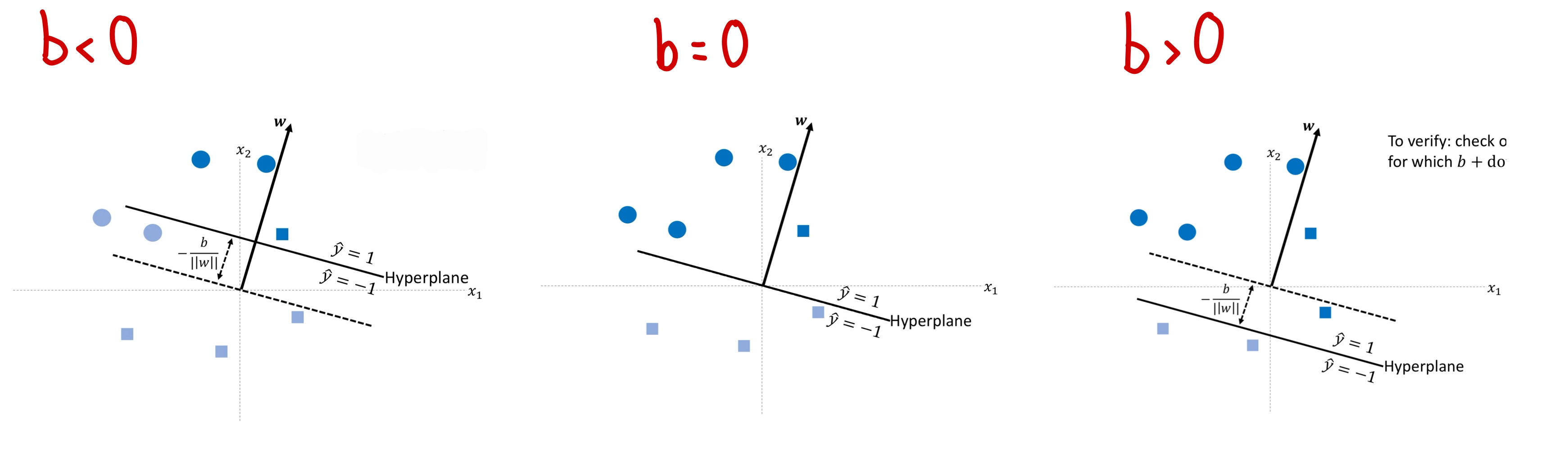
A negative $b$ shifts the boundary in the direction of $\mathbf{w}$; a positive $b$ shifts it against $\mathbf{w}$. When $b=0$, the hyperplane passes through the origin.

Regression mode

Remove the sign function and the same neuron becomes a linear regressor:

$\hat{y}=b+{\sum }_{i=1}^D{w}_i{x}_i=b+\mathbf{w}\cdot \mathbf{x}$

This is standard linear regression ($y=mx+c$ in 1D). The weight $w_i$ is the slope along dimension $i$ and $b$ is the intercept. Instead of splitting space into two half-spaces, the neuron now fits a line (or hyperplane) through the data.

Hard vs soft perceptron

The version above — with the sign activation — is called a hard perceptron. The output flips abruptly from $-1$ to $+1$ at the decision boundary: the decision is “hard”. A soft perceptron replaces the sign with a smooth activation like the sigmoid function:

$\hat{y}=\sigma \left(b+\mathbf{w}\cdot \mathbf{x}\right)\in (0,1)$

Output transitions smoothly through the boundary instead of stepping; the decision is “soft”, and the value can be read as a probability $p(y=1\mid \mathbf{x})$.

	Hard perceptron	Soft perceptron
Activation	sign $\text{sgn}(z)$	sigmoid $\sigma (z)$ (or tanh, ReLU, …)
Output	$\{-1,+1\}$	$(0,1)$
Transition at boundary	Step	Smooth S-curve
Differentiable?	No — derivative is 0 almost everywhere, undefined at 0	Yes — derivative is positive and well-defined
Trainable by gradient descent?	No — $\nabla L\equiv 0$, parameters never update	Yes

The whole distinction reduces to one property: differentiability. The hard perceptron’s sign function has derivative zero, so by the chain rule the loss gradient collapses to the zero vector and gradient descent cannot move the parameters. Soft activations have non-zero gradients, so training works. Every other apparent difference (probability interpretation, smooth output, gradient flow through deeper layers) is a downstream consequence of that one fact.

This is why every neuron in a modern neural network is a soft perceptron. “Hard” is the original Rosenblatt-1958 model; “soft” is what we use whenever we actually need to train. See multi-layer-perceptron (built from soft perceptrons) and sigmoid function (the canonical soft activation).

Limitations

A single perceptron can only produce a linear decision boundary. If the data is not linearly separable — for instance, an XOR-like pattern where positive points appear in opposite corners — no single hyperplane can classify it correctly. Solving non-linearly separable problems requires combining multiple perceptrons into layers, leading to multi-layer perceptrons (MLPs) and backpropagation (week 3).

Worked Example

Given $\mathbf{w}=(1,1,3)$ and $b=2$, classify $\mathbf{x}=(-1,-1,-3)$:

1. Compute the weighted sum: $\mathbf{w}\cdot \mathbf{x}=(1)(-1)+(1)(-1)+(3)(-3)=-1-1-9=-11$
2. Add bias: $-11+2=-9$
3. Apply sign: $\text{sgn}(-9)=-1$

So $\hat{y}=-1$.

For $\mathbf{x}=(0,0,1)$: $\mathbf{w}\cdot \mathbf{x}+b=3+2=5>0$, so $\hat{y}=+1$.

Related

• dot-product — the algebraic operation at the heart of the perceptron
• decision boundary — the geometric object the perceptron defines
• loss-function — how we measure whether the perceptron’s parameters are good

Active Recall

What changes when you remove the sign function from a perceptron, and what kind of problem does it now solve?

Without the sign function, the perceptron outputs the raw value $b+\mathbf{w}\cdot \mathbf{x}$ — a continuous number rather than $\pm 1$. This turns it into a linear regressor that fits a line (or hyperplane) through data, predicting continuous targets like commute time or house price.

A perceptron has $\mathbf{w}=(0,1)$ and $b=-1$. What does its decision boundary look like geometrically, and which points get classified as $+1$?

The boundary is $0\cdot x_1+1\cdot x_2-1=0$, i.e. the horizontal line $x_2=1$. Points above this line ($x_2>1$) are classified as $+1$; points below as $-1$. The weight vector points straight up, so the boundary is horizontal.

Why can't a single perceptron solve the XOR problem, and what architectural change is needed?

XOR has positive examples at $(-1,-1)$ and $(1,1)$, and negative examples at $(-1,1)$ and $(1,-1)$ — opposite corners. No single straight line can separate them. You need at least two perceptrons in a first layer (each drawing its own boundary) whose outputs feed into a third perceptron, forming a multi-layer network.

What is the difference between a hard perceptron and a soft perceptron, and which property is the distinction really about?

A hard perceptron uses the sign activation: output is $\pm 1$ with an abrupt step at the decision boundary. A soft perceptron uses a smooth activation (sigmoid, tanh, ReLU, …): output is a continuous value with a smooth transition. Everything else (probability interpretation, smooth output) follows from the underlying property: differentiability. The hard perceptron’s sign function has derivative zero almost everywhere, so gradient descent collapses to $\nabla L=0$ and the parameters never update. The soft version has a non-zero gradient and can actually be trained — which is why every modern neural network neuron is a soft perceptron.

In the biological analogy, what do dendrites, synaptic strengths, and the axon correspond to in the perceptron model?

Dendrites correspond to the inputs $x_i$ (receiving signals from other neurons). Synaptic strengths correspond to the weights $w_i$ (how much each input matters). The axon corresponds to the output $\hat{y}$ (the signal sent onward after the soma aggregates and thresholds).

Compute the output of a perceptron with $\mathbf{w}=(2,-1)$, $b=0$ for input $\mathbf{x}=(3,6)$. Explain the geometric meaning.

$\mathbf{w}\cdot \mathbf{x}+b=(2)(3)+(-1)(6)+0=6-6=0$. The sign function at $0$ gives $-1$ (by convention, $\text{sgn}(0)=-1$). Geometrically, the point lies exactly on the decision boundary $2x_1-x_2=0$, which is the line $x_2=2x_1$.