A small window of weights slid across the image, computing dot products. The same weights apply at every spatial position — that’s weight sharing — and that’s what makes processing images tractable.
What is a kernel (and a filter)?
A kernel is a small grid of numbers — typically or — that you slide across the input. The numbers inside it are weights: the same kind of learnable parameters as in any other neural network layer. A kernel is to a convolution what a weight vector is to a perceptron: the thing whose values determine what the operation computes.
The word filter is used almost interchangeably with kernel, with one common convention:
- Kernel refers to the 2D grid of weights — e.g. a single slice.
- Filter refers to the full set of weights for one output channel, including the depth dimension. For a colour image with 3 input channels, a filter is actually weights — three stacked kernels, one per input channel, that act together to produce one output channel.
In practice — and in these notes — the two words are often used as synonyms, and which one is “right” depends on the context. When the depth doesn’t matter (e.g. a grayscale image or a generic 2D illustration), say kernel. When you mean the whole 3D weight tensor that produces one output map, say filter. If a sentence works with either, don’t worry about the distinction.
The operation
Given a 2D input of shape and a 2D kernel of shape , the convolution at output position is:
Place the kernel on top of the image, centred at . Multiply elementwise, sum the results, write down a single number. Slide the kernel one step, repeat. Cover the whole image and you’ve produced a 2D output.
This is exactly the perceptron’s dot product — applied to a small image patch instead of the whole input vector. The bias is added once per kernel application (omitted from the formula above for brevity, but always present in practice).
ASIDE — Mathematician's vs computer scientist's convolution
Strict mathematical convolution has a kernel flip — instead of . In CNN libraries (PyTorch, TensorFlow) the un-flipped form is used and still called “convolution” (technically cross-correlation). The difference doesn’t matter for learning: the network just learns whatever kernel orientation works, flipped or not. We use the un-flipped form throughout.
TIP — Convolution outside neural networks
Convolution isn’t a CNN-specific invention; it’s a general operation that combines two lists (or two functions) into a third list, where each output element is some sum of pairwise products. You’ve already seen it in disguise:
- Multiplying two polynomials. The coefficients of the product are convolutions of the coefficients of the inputs.
- Long multiplication. When you multiply two numbers digit-by-digit (units × units, units × tens, …) and add up the results aligned by place value, you’re computing a convolution of their digit sequences.
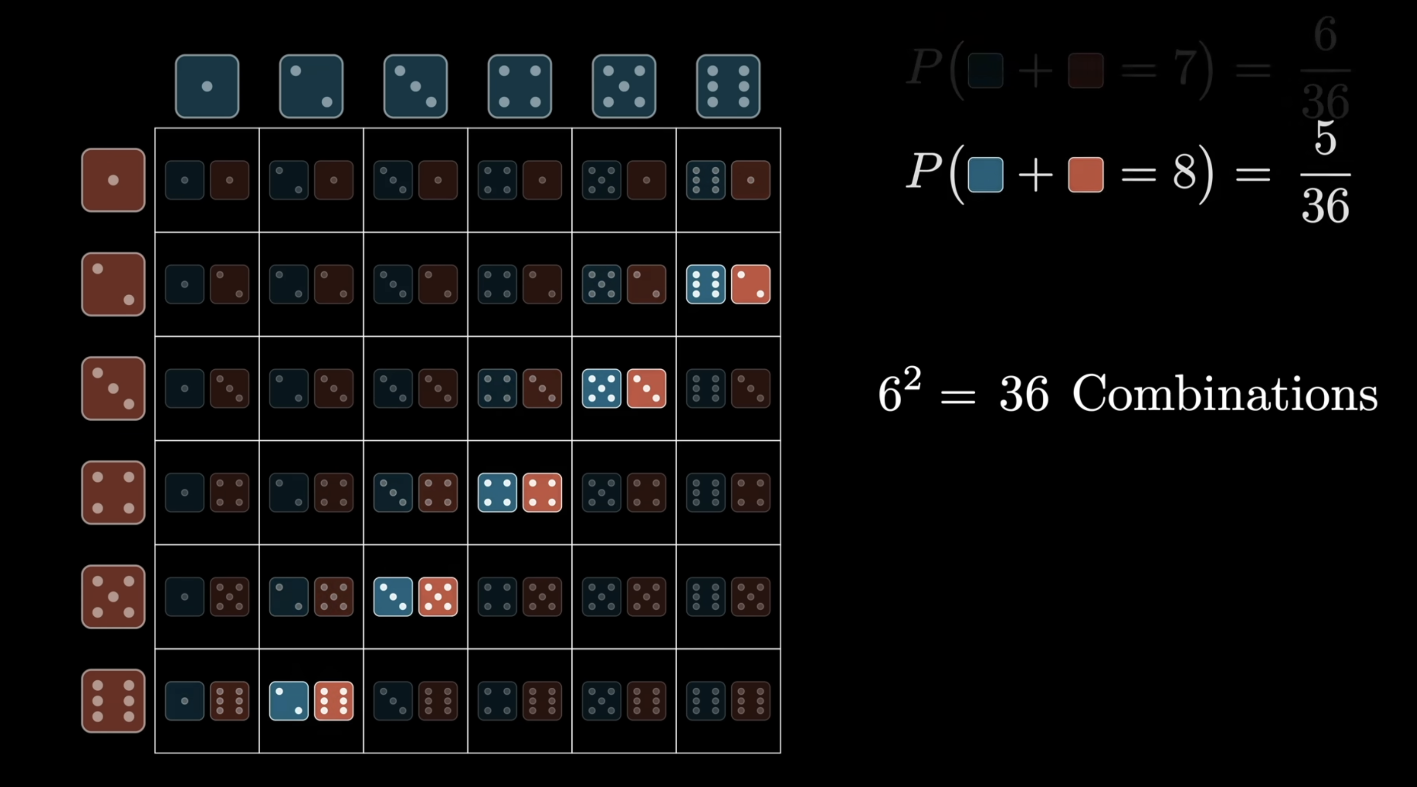
- Sum of two dice. The probability distribution of for two independent dice is the convolution of each die’s distribution. Visualise it as the multiplication table of all pairwise products, summed along diagonals.
Each diagonal of the table corresponds to one outcome of — e.g. all the ways to roll a sum of 8 lie on one diagonal. Summing the cells along that diagonal gives . That diagonal-sum-of-products is the convolution operation; the image-kernel version above is exactly the same idea, just in 2D.
The CNN view — sliding a kernel over an image — is the same operation specialised to 2D inputs and a small finite kernel. Image convolution is a particular instance of this much older mathematical idea.
ASIDE — Fast convolution via FFT
Naive convolution of two length- sequences takes time (each output element is a sum over pairwise products). For very long sequences this is prohibitive. The Fast Fourier Transform (FFT) gives an algorithm: take the FFT of both inputs, multiply the transforms point-wise, take the inverse FFT. The reason this works connects to the polynomial-multiplication view of convolution.
For CNN-style 2D convolution with small kernels (e.g., ), the kernel is so small that direct computation is already fast and FFT-based methods don’t help. But for some specialised image-processing tasks — large kernels, or repeated convolutions in scientific computing — FFT-based convolution is the standard.
What convolution is doing, intuitively
A dot product is a similarity measure: , large and positive when two vectors point similarly, near zero when orthogonal, large and negative when opposed. Apply this to convolution: the output value at position is large when the local image patch around looks like the kernel.
So convolution scans the image asking “where does this pattern appear?” and the output map records the answers spatially. A bright pixel in the output map indicates “the pattern is here”; a dark pixel says “not here”.
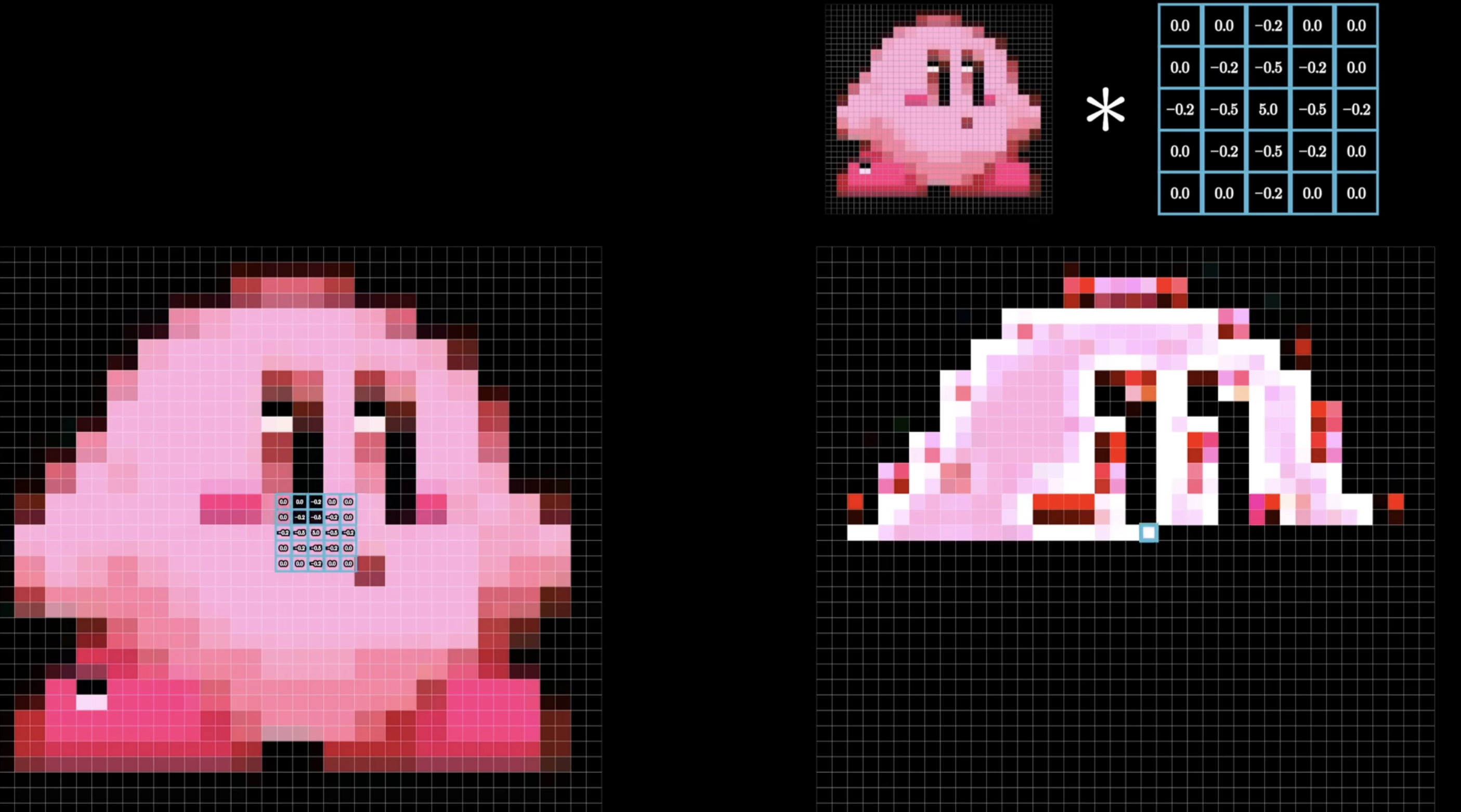
The kernel above is an edge-detection filter (positive centre, negative neighbours, zero outer ring — sums to zero). Applied to the cartoon character on the left, the output on the right lights up exactly where intensity changes — i.e. along the silhouette and internal edges. That bright skeleton is the answer to “where does this kernel’s pattern appear in the image?”
TIP — Convolution as feature extraction
A kernel is a small recognisable pattern: a vertical edge, a horizontal edge, a corner, a circular dot. The output map shows where in the image those patterns occur. That’s why convolution is called feature extraction: the kernel defines a feature, and convolution detects every place where it shows up.
Hand-designed vs learned kernels
Convolution predates neural networks. For decades, image-processing researchers designed kernels by hand to extract specific features:
| Kernel | Effect |
|---|---|
| Identity (output = input) | |
| Sobel — horizontal edge detection | |
| Sobel — vertical edge detection | |
| Sharpen | |
| Box blur (3×3 average) | |
| Edge detection (omnidirectional) |
These were human-designed. Researchers spent months tuning kernels for one feature.
TIP — Reading a kernel from its weights
A useful heuristic: look at what the kernel weights sum to.
- Sum to 1 (e.g., box blur, Gaussian blur) — preserves average brightness. The output is a smoothed version of the input.
- Sum to 0 (e.g., Sobel, Laplacian) — averages of constant regions cancel to zero, so the output is zero in flat regions and only “lights up” where intensity changes. That’s edge detection.
- Sum > 1 with negative neighbours (e.g., the sharpen kernel above, sum = 1 with a centre weight of 5 against 4 neighbours of ) — boosts a pixel relative to its neighbours, accentuating local contrast.
The pattern of signs and magnitudes inside the kernel tells you what feature it responds to; the sum tells you whether it preserves brightness or measures change.
The CNN innovation: make the kernel a vector of learnable parameters, just like any other weight. The network discovers, end-to-end, whatever kernel best helps the loss go down. No more hand-design. Filtering becomes part of the training loop.
This is what people mean when they call CNNs end-to-end machine learning: you hand the network the raw image and the loss, and it figures out — on its own — which kernels are worth applying to extract the features that drive the loss down. The architecture is designed by humans; the kernels are learned by the machine. What used to be months of human kernel-tuning becomes a few epochs of gradient descent.
Weight sharing
The single most important property of a convolution layer is that the same kernel weights are reused at every spatial position of the input. One kernel, applied everywhere. That’s weight sharing.
Why an MLP is wasteful for images
Recall the chef analogy from multi-layer-perceptron. In a fully connected MLP, every chef in the next layer has their own recipe with one weight per pixel. For a image fed into a hidden layer with chefs:
- 1,000,000 ingredients on the counter (one per pixel)
- 1,000,000 chefs, each with a recipe of length 1,000,000
- Total weights: — one trillion
The parameter count is only half the problem. The bigger issue is the network has to learn the same thing many times over. Train a chef who specialises in detecting a cat in the top-left, then move the cat to the centre — the top-left chef sees only background and learned nothing useful for this new image. A different chef has to learn cat-detection from scratch in each new position.
This is wasteful because a cat in the top-left and a cat in the centre look the same — same edges, same curves, same textures. The MLP forces the network to rediscover this fact by example at every position, instead of building it into the architecture.
Two structural facts about images
Images have two properties any sensible architecture should exploit:
- Features are local. Detecting an “edge” or a “corner” only needs a small neighbourhood — typically or pixels. The whole image is irrelevant for that decision.
- Features are translation-invariant. A horizontal edge looks the same whether it sits at the top or the bottom of the image. The detector for it doesn’t change with position.
These two facts together suggest a wildly different architecture: one small chef whose recipe gets applied at every position of the image.
One chef walking the image (= one convolution kernel)
Forget the army of MLP chefs. Picture one chef with a tiny recipe — 9 weights. Instead of looking at the whole image at once, they:
- Stand over a patch (say the top-left corner).
- Apply their recipe to the 9 pixels they see — a dot product.
- Write down one number — “how strongly did my recipe activate here?”
- Step one pixel to the right.
- Repeat across the whole image.
The chef produces a 2D output map: each cell records how much their recipe matched the patch at that position. The chef has 9 weights total — not 9 per position. The same 9 weights are reused at every location. That’s weight sharing, and the sliding-recipe operation is convolution.
What weight sharing buys you
Four wins, all huge:
- Massive parameter savings. A kernel is 9 numbers (or on a depth- input) — typically 9 orders of magnitude fewer than the FC alternative. (Concrete numbers in Why this is so much cheaper than full connectivity below.)
- The kernel becomes a feature detector. A specific pattern of kernel weights responds to a specific pattern in the image. A recipe with “+1 on top, 0 in middle, -1 on bottom” lights up exactly where bright-above-dark-below transitions occur — i.e. horizontal edges. The output map answers “where in the image does this feature appear?”
- Translation equivariance. Because the same detector is used at every position, a feature that activates the kernel at one location activates it identically at any other. Move the cat ten pixels to the right and the activations move ten pixels to the right — automatically, without the network having to learn this from data. See shift-invariance-equivariance.
- Far more training signal per weight. In an MLP, each weight only ever receives gradient signal from one (input pixel, neuron) pair. In a convolution, every position in every image contributes a gradient update to the same shared weight. One kernel weight effectively gets gradient signal from every spatial location of every training image — orders of magnitude more learning per parameter. This is why CNNs train successfully with far less data than equivalent MLPs would need.
One kernel detects one pattern — use many
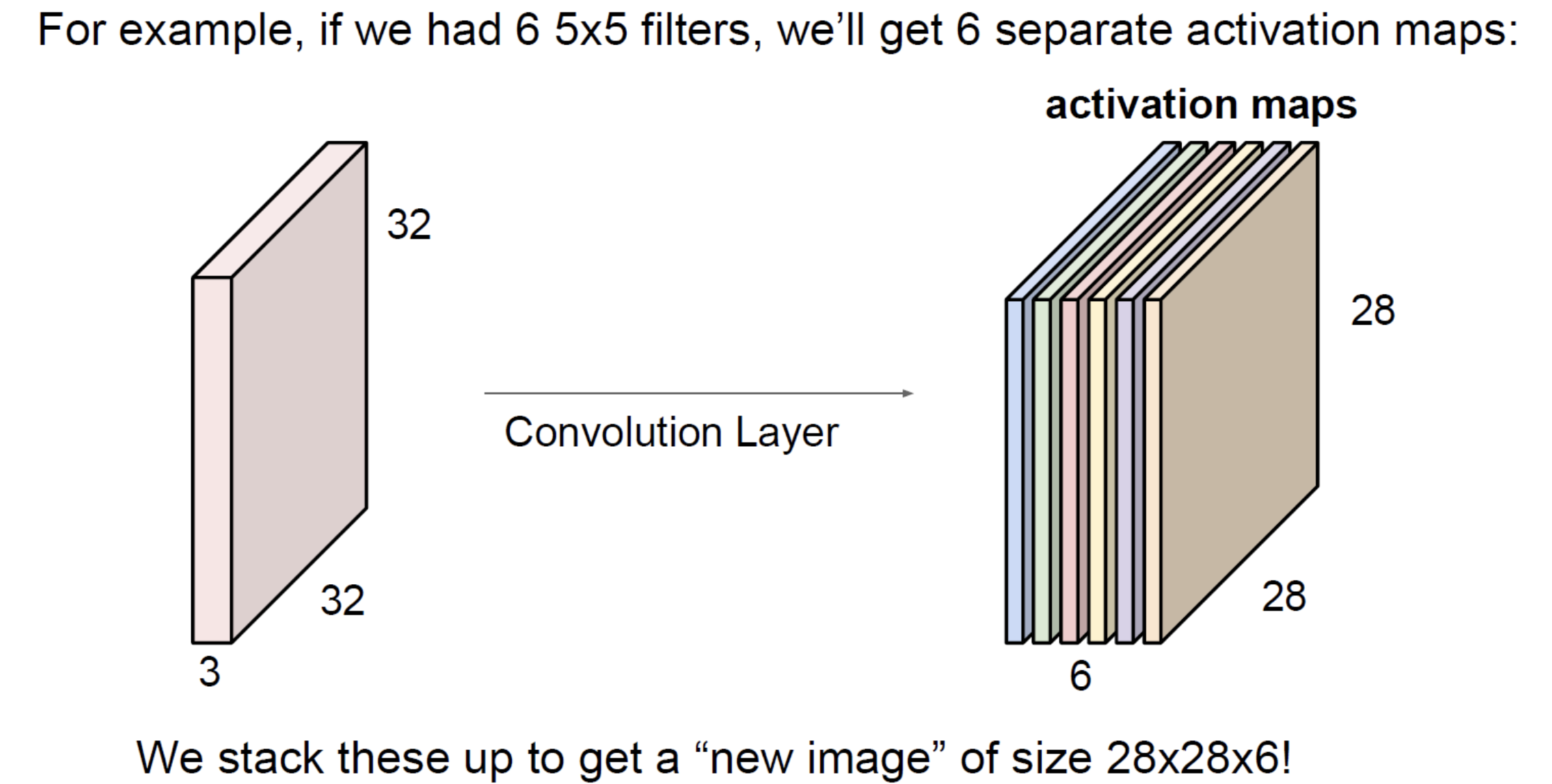
A single kernel can only respond to one feature. Real images need many: horizontal edges, vertical edges, curves, dots, textures, colour blobs.
The fix is multiple kernels in parallel. If the layer has kernels, that’s chefs each scanning the whole image with their own recipe. Each produces a separate 2D output map. The layer’s output is a stack of feature maps — shape . This is what makes “convolution layer” a layer in the neural-network sense: an operation parameterised by filters that takes a 3D input volume and returns a 3D output volume.
Stacking layers → CNN
The final step is to stack convolution layers. Layer 2’s chefs don’t have to look at raw pixels — they can look at layer 1’s feature maps:
- Layer 1 chefs see raw pixels → learn low-level features (edges, dots, simple textures).
- Layer 2 chefs see layer 1’s edge/dot maps → learn mid-level features (corners, simple shapes, textures).
- Layer 3 chefs see layer 2’s corner/texture maps → learn parts (eyes, wheels, leaves).
- Layer 4 chefs see layer 3’s part maps → learn objects (faces, cars, trees).
Each layer applies the same primitive — a stack of shared small kernels scanning whatever is on the counter — but operates on progressively more abstract feature maps. The compositional hierarchy emerges naturally because every layer can build on the previous one’s outputs. The chefs at every level still just do “weighted sum of nearby ingredients, then bake” — the only thing that changes is what the ingredients mean.
A convolutional neural network is exactly this: stacked convolution layers with activation-functions between them, pooling for spatial downsampling, eventually feeding into a small fully connected classifier at the end. See convolutional-neural-network for the full architecture story.
The constrained-MLP view
Weight sharing is also why convolution can be viewed as a constrained MLP: take a fully connected layer and force (i) most weights to be zero (local connectivity — only nearby input pixels contribute), and (ii) the remaining weights to be tied across spatial positions (weight sharing). The result is a convolution. The “constraint” encodes a prior — features are local and the same features appear everywhere — that perfectly matches how images work.
The three hyperparameters of a convolution
Every convolution layer is fully specified by three numbers:
- Kernel size . The spatial dimensions of the filter — typically or . This sets the receptive field of one output pixel: how large a patch of the input each output value sees.
- Stride . The step size, in pixels, when sliding the kernel across the image. visits every position; skips every other position and halves the output resolution.
- Padding . The width of the zero border added around the input before convolving. Padding lets the kernel be centred on the boundary pixels, which would otherwise be lost. Note: “padding 1” means the border is 1 pixel wide — the value of those pixels is still 0; the “1” describes thickness, not intensity.
These three knobs together determine the output size.
Output size: the magic formula
Naive convolution shrinks the output. A 3×3 kernel on a 7×7 image gives a 5×5 output: the kernel can’t be centred on the boundary pixels, so one row/column is lost on each side. Two of the three hyperparameters above — padding and stride — let you control this:
- Padding — pad the input with zeros around each border before convolving.
- Stride — step size when sliding the kernel ( visits every position, skips every other).
The magic formula captures the result. For input width , kernel size , stride , padding :
(Same formula for height with and .) For the output volume to be a clean grid, this fraction must be an integer.
Common settings
| Setting | Output size relative to input | |||
|---|---|---|---|---|
| Same convolution (3×3) | 3 | 1 | 1 | — no shrinkage |
| Same convolution (5×5) | 5 | 1 | 2 | |
| Valid convolution (3×3) | 3 | 1 | 0 | — shrinks by 2 |
| Strided (3×3) | 3 | 2 | 1 | — halves |
The general “same convolution” rule for an odd kernel: .
A image is convolved with a kernel using stride 1 and padding 0. What size is the output?
. Output is .
We want a kernel to produce an output the same spatial size as the input. What padding should we use, with stride 1?
. Pad with 2 zero rows/columns on each side. Then .
A image is convolved with a kernel and stride 3, no padding. Why is this configuration awkward?
, which isn’t an integer. The kernel can’t tile the image cleanly with that stride: positions visited are 1, 4, 7 along each dimension, but at column 7 the kernel only has 1 column of input remaining on its right, not 3. Either truncate the operation (lose information) or change one of , , so the magic formula gives an integer.
Convolution in the depth direction
Real images have channels: RGB has 3, intermediate feature maps in a CNN can have hundreds. A convolution kernel always extends through the full input depth.
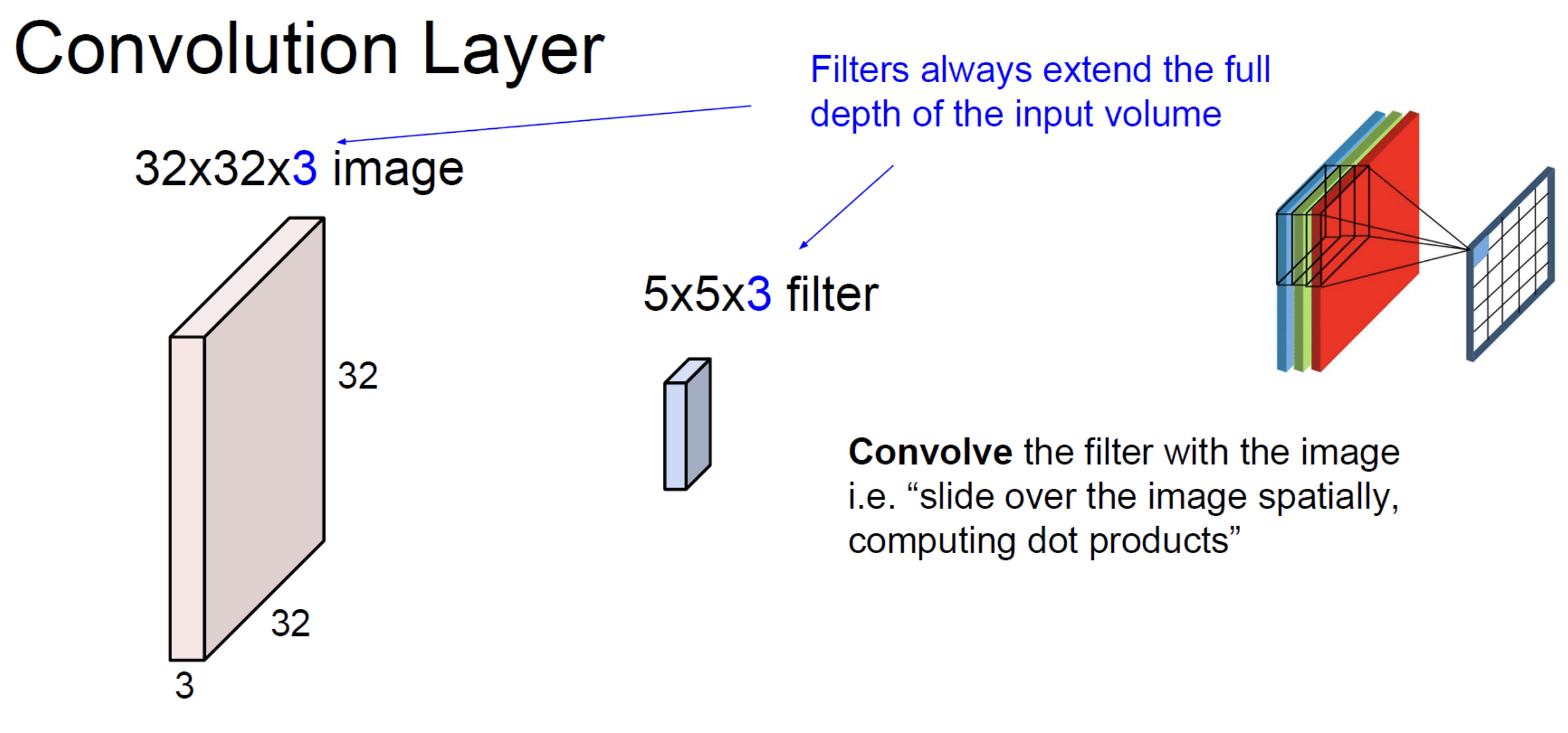
For a 2D input , each kernel has shape — same depth as the input. The dot product is over the entire patch ( elements per kernel). The output of one such kernel is a 2D map (one channel).
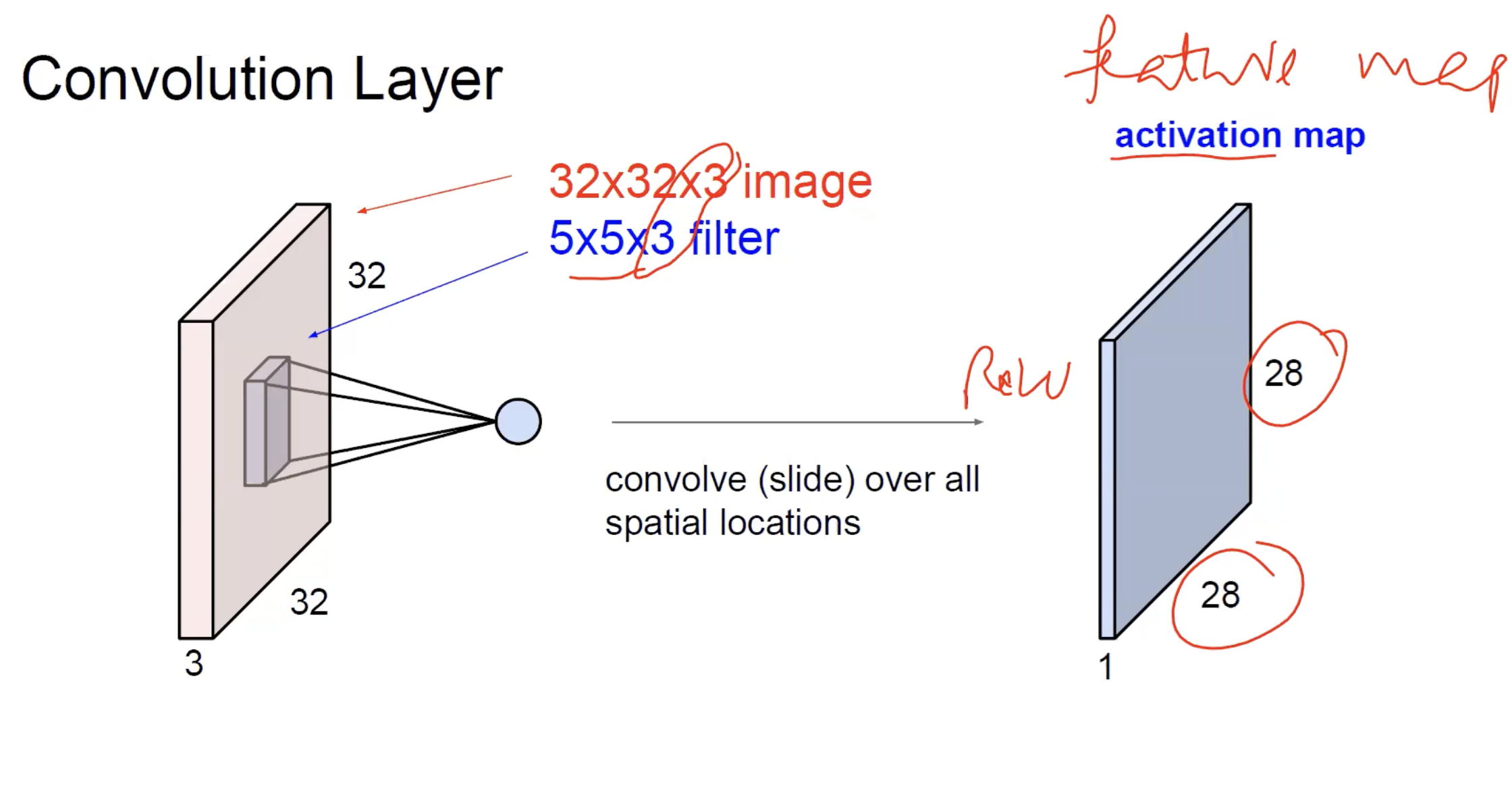
The result of sliding one filter over a image is a single activation map — the output’s spatial extent is set by the magic formula, the depth is 1 (one filter, one map).
To get a multi-channel output, use multiple kernels. kernels in parallel produce a stack of 2D maps, depth . That’s why a convolution layer’s output volume has dimensions — the depth equals the number of kernels, set independently by the layer designer.
See convolutional-neural-network for how this stacks up into a full network.
Why this is so much cheaper than full connectivity
Compare a fully connected layer and a convolution layer for the same input:
Input: image (3072 values).
Fully connected layer to 1000 hidden units: weights.
Convolution layer with 64 kernels of size : weights.
Three orders of magnitude difference, despite the conv layer producing a much richer (multi-channel, spatially structured) output. The savings come entirely from weight sharing: the same kernel weights are reused at every spatial position, instead of having a unique weight per (input, output) pair.
This scaling is why CNNs work and MLPs don’t, on real images. See image-representation for why MLPs hit a parameter wall.
Padding and information at the borders
Padding fills the input border with zeros (the most common choice; “reflect” and “replicate” padding also exist) so the kernel can centre on boundary pixels.
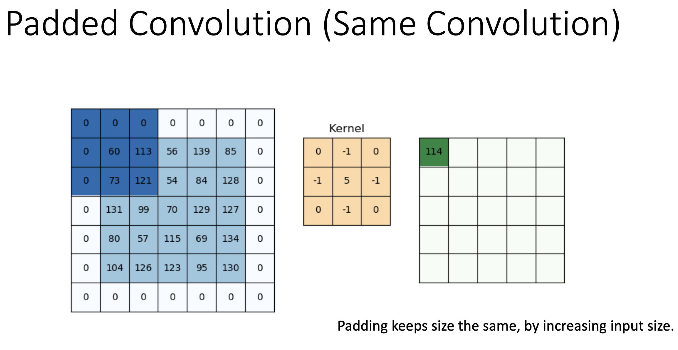
Concrete example: a image padded with a one-pixel zero border becomes . A kernel can now centre on the original corner pixel — the top-left output value is the dot product of the kernel with a patch that includes the padded zeros on two sides. The output is back to , the same size as the original input. That’s “same convolution”.
- Without padding: every output pixel is computed from a real patch of the input; output is smaller.
- With padding: output is the same size, but boundary outputs are computed from patches partly filled with zeros.
TIP — "Padding 1" doesn't mean the value 1
When the slides say “padding ”, that’s the width of the border in pixels — one row of zeros added at the top, one at the bottom, one column at the left, one at the right. The value of those padding pixels is still 0 (zero-padding); the “1” refers to the thickness of the added border, not its intensity.
There’s a quality tradeoff: boundary outputs are slightly less reliable (the zero pixels contribute spurious information), but you avoid losing data at the edges of every layer. Modern CNNs almost always use padding to maintain spatial size through the conv layers, then explicitly downsample with pooling when reducing resolution is desired.
Stride and downsampling
A convolution with stride 2 produces a halved output. This is one way to reduce spatial size. The other way is pooling. Modern architectures use both: strided convolutions in some places (e.g., the first layer of ResNet) and pooling in others.
Higher strides skip more positions, which loses information faster. Stride 1 is the default.
Related
- perceptron — convolution is a perceptron applied to a local patch, with weights reused across patches
- dot-product — the per-position operation, which doubles as a similarity measure
- convolutional-neural-network — the architecture built by stacking convolution layers
- pooling — the other downsampling primitive in CNNs
- image-representation — explains the input that convolution operates on
- backpropagation — convolution is differentiable; its gradient is computed efficiently using the same chain-rule machinery
Active Recall
Write down the convolution formula for a 2D input and explain what each term means.
. Place the kernel on top of the image , centred at . Multiply the kernel elementwise with the local image patch and sum — that’s one output pixel. Slide and repeat to build the full output map .
A convolution layer has 64 kernels of size applied to a input. How many learnable parameters does it have, and what is the output spatial size with padding 1, stride 1?
Each kernel has weights plus 1 bias = 28 parameters. With 64 kernels: parameters. Output spatial size: — same as input (this is “same convolution”). Output volume is .
What does it mean to say convolution "shares weights"? What is the alternative, and why is it infeasible for images?
The same kernel — a small set of weights — is applied at every spatial position. The alternative is a fully connected layer where every (input pixel, output unit) pair has its own weight. For a image with hidden units, the FC layer needs weights (one trillion); the conv layer with a kernel and 64 filters needs about 600 — roughly nine orders of magnitude fewer. Image-scale FC layers don’t fit in memory, can’t be trained, and don’t have enough data to fit anyway.
Why does convolution naturally encode "this pattern appears somewhere" without learning a separate detector for every position?
Because the same kernel weights apply at every spatial position. If the kernel’s pattern matches a patch at position , the same kernel will also match the same pattern at , , etc. — without any separate parameters. The output map’s value tells you where the pattern is. This is why CNNs handle objects in different parts of an image more gracefully than MLPs do.
Two stacked convolutions vs one convolution. Which has more learnable parameters, and which has a larger receptive field?
A single kernel: weights per filter (where is input depth), receptive field 5×5. Two stacked kernels: weights per filter (where is the depth between the two layers), receptive field 5×5 (each layer adds 2 to the receptive field on each side). For comparable depths, two has fewer weights and the same receptive field — plus an extra non-linearity in between, which adds expressiveness. This is why VGG uses kernels exclusively.
What's the difference between "valid" and "same" convolution? Give an example of each for a 3×3 kernel on a image.
Valid: no padding (). Output size , so . Same: padding chosen to preserve size (). Output size , so — same as input.