gradient-descent-nc

The workhorse algorithm of machine learning: start with random parameters, compute the slope of the loss at that point, take a small step downhill, repeat.

Motivation: measuring badness isn’t enough

Week 1 gave us a loss-function — a way to score how bad the current parameters are. But telling a model how badly it’s doing is not the same as telling it what to change to do better. We need a mechanism that turns the loss measurement into a prescription for updating each parameter. Gradient descent is that mechanism.

Formally, gradient descent is a local search technique for minimising a cost function. “Local” because at any point in parameter space it only looks at the slope right there and takes one small step — it has no global map of the landscape.

The loss is typically a sum or average over all training samples (e.g. $L={\sum }_j(y^j-{\hat{y}}^j{)}^2$). So each gradient step doesn’t just improve performance on one example — it pushes the parameters toward better performance across the whole training set at once. Every sample contributes to every update. (This is also why vanilla GD is expensive for large datasets; stochastic and mini-batch variants estimate the gradient from a subset instead — see gradient-descent-variants.)

The core equation

You should know this by heart:

${\mathbf{\theta }}^{t+1}={\mathbf{\theta }}^t-\eta \nabla L_t$

• ${\mathbf{\theta }}^t$ — the current parameter vector (e.g. $(w_1,w_2,\dots ,b)$)
• $\nabla L_t$ — the gradient of the loss-function at ${\mathbf{\theta }}^t$
• $\eta$ — the learning-rate (a hyperparameter)
• Minus sign — the gradient points uphill, so we negate it to walk downhill

The algorithm is:

1. Initialise ${\mathbf{\theta }}^0$ randomly.
2. Compute $\nabla L_t$.
3. Update ${\mathbf{\theta }}^{t+1}={\mathbf{\theta }}^t-\eta \nabla L_t$.
4. Repeat until convergence or a max iteration count.

Why it works: the slope tells you which way is down

The gradient $\nabla L$ is a vector of partial derivatives — one component per parameter:

$\nabla L({\mathbf{\theta }}^t)=\left(\begin{array}{c}\frac{\partial L}{\partial w_1}\\ \frac{\partial L}{\partial w_2}\\ ⋮\\ \frac{\partial L}{\partial b}\end{array}\right)$

From calculus, the gradient points in the direction of steepest increase. Negating it gives the direction of steepest decrease — which is exactly what minimising the loss requires. The learning rate $\eta$ controls how far along that direction to step.

TIP — The blindfolded hiker analogy

Imagine someone blindfolded on a hillside who wants to reach the valley. They can’t see, but they can feel the slope under their feet. They step in whichever direction goes downhill, and repeat. Gradient descent is exactly this — the loss landscape is the hill, the gradient is the slope they feel, and $\eta$ is the length of each step.

The analogy also explains why the loss must be smooth: a ball can only roll down a smooth hill. If the surface is kinked or discontinuous (as with the sign function), there’s no well-defined slope to follow — the ball gets stuck or stops at flat steps. Smoothness is what makes the landscape rollable.

The 1D picture

In one dimension the algorithm collapses to a simple rule. Compute the slope $dL/d\hat{x}$ at your current point:

• Slope positive → function is increasing → step left (decrease $\hat{x}$).
• Slope negative → function is decreasing → step right (increase $\hat{x}$).

The update ${\hat{x}}^{t+1}={\hat{x}}^t-\eta \cdot dL/d\hat{x}$ encodes both cases in one expression: the minus sign automatically inverts the direction of the slope.

Worked example: 1D with absolute error

Take the loss-function $L(\hat{x},\mathbf{x})={\sum }_i|x_i-\hat{x}|$ with measurements $x_1=19$, $x_2=17$, $x_3=24$. Starting from ${\hat{x}}^0=24.5$ with $\eta =1$:

$t$	${\hat{x}}^t$	$\nabla L_t$	${\hat{x}}^{t+1}={\hat{x}}^t-\eta \nabla L_t$
0	24.5	$1+1+1=3$	21.5
1	21.5	$1+1-1=1$	20.5
2	20.5	$1+1-1=1$	19.5
3	19.5	$1+1-1=1$	18.5
4	18.5	$-1+1-1=-1$	19.5

The true optimum is ${\hat{x}}^{\ast }=19$ (the median, for absolute error). Notice the last two rows — the estimate gets stuck oscillating between $18.5$ and $19.5$. This is exactly the symptom of a learning rate that’s too large for the neighbourhood of the optimum.

Why the gradient?

Of all the directions you could step in, why is the gradient the one to follow? Because multivariable calculus gives you a theorem for free: the gradient $\nabla L$ points in the direction of steepest ascent of $L$, and its length $\Vert \nabla L\Vert$ is the rate of change in that steepest direction. No other unit direction increases the function faster at that point. By symmetry, $-\nabla L$ is the direction of steepest descent — the single best choice for minimisation.

Concretely, the gradient is just a vector of partial derivatives:

$\nabla L(w_1,\dots ,w_D,b)=\left(\begin{array}{c}\partial L/\partial w_1\\ \partial L/\partial w_2\\ ⋮\\ \partial L/\partial b\end{array}\right)$

Each partial derivative $\partial L/\partial w_i$ answers a simple question: how much does the loss change if I nudge $w_i$ a tiny bit, holding everything else fixed?. Stacking all these local sensitivities into one vector gives you the gradient.

A non-spatial way to read the gradient

Picturing the gradient as an arrow in a high-dimensional parameter space is hard. A more useful reading — especially for networks with millions of parameters — is to think of $-\nabla L$ as a list of per-parameter instructions. Each component $-\partial L/\partial w_i$ tells you two things:

1. Sign — should $w_i$ be nudged up or down?
2. Relative magnitude — how much does this particular parameter matter? A component with a large magnitude means that parameter is currently pulling a lot of weight on the loss; nudging it will change the loss a lot. A component close to zero means the parameter barely matters right now.

So $-\nabla L$ is a prioritised to-do list for the parameters: tweak these weights in these directions, and give more push to the ones that will move the loss the most.

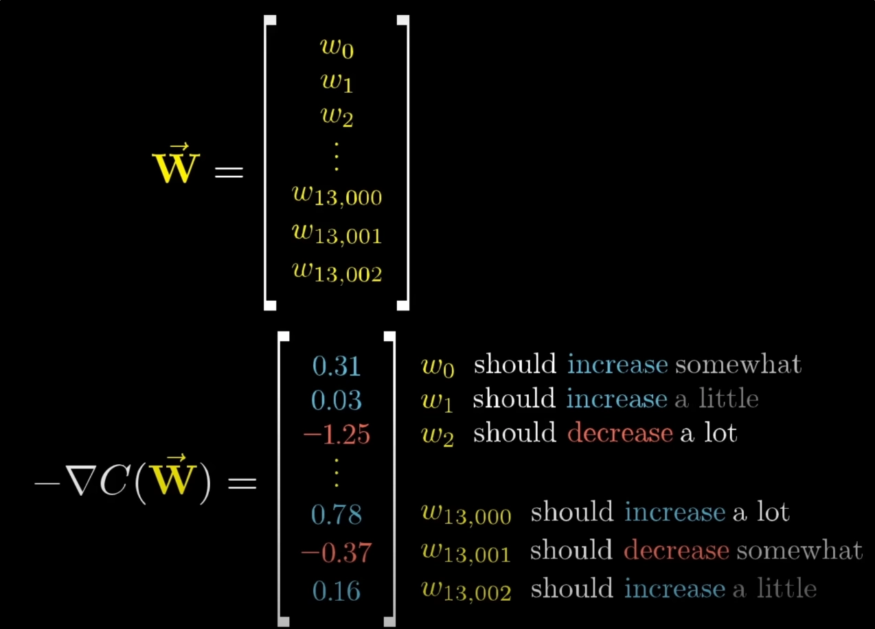
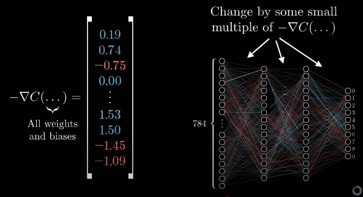
Bang for your buck. In a network with 13,002 weights and biases (say), the gradient encodes the relative importance of each one at the current point in training. Changing one weight might barely move the loss; changing another might move it a lot. The gradient tells you which is which, automatically.

TIP — Self-correcting step sizes near a smooth minimum

For smooth losses (e.g. squared error, cross-entropy), the gradient magnitude naturally shrinks as you approach the minimum — the slope flattens out. Because the update is $\eta \nabla L$, the step size shrinks with it, slowing the optimiser automatically and helping it settle without overshooting.

This fails for non-smooth losses like absolute error: the gradient magnitude stays fixed (it’s $\pm 1$ on each side of a kink) right up to the minimum, so the step size doesn’t shrink and you oscillate — exactly what happens in the worked example above. Smooth, convex losses are forgiving; kinked losses are not.

Worked example: 2D regression on penguin counts

The 1D toy example uses a single parameter, but real models have many. Here’s the same algorithm applied to a two-parameter linear regression — a much closer analogue of how it’s used in practice.

Three penguin counts taken on an island: 332 in 2010, 353 in 2012, 419 in 2016. Re-express the year as “years since 2010”, so the data is $(0,332),(2,353),(6,419)$.

Fit a linear model $\hat{y}=wx+b$ with squared or absolute error loss; here we use absolute error. Initialise $w^0=10$, $b^0=350$, learning rate $\eta =0.5$.

Forward (loss):

Sample	$x_i$	$y_i$	${\hat{y}}_i=10x_i+350$	${\hat{y}}_i-y_i$	$\Vert {\hat{y}}_i-y_i\Vert$
1	0	332	350	$+18$	$18$
2	2	353	370	$+17$	$17$
3	6	419	410	$-9$	$9$

Total loss $L=18+17+9=44$.

Gradient. For absolute error, $\partial |{\hat{y}}_i-y_i|/\partial w=\text{sign}({\hat{y}}_i-y_i)\cdot x_i$ and $\partial |{\hat{y}}_i-y_i|/\partial b=\text{sign}({\hat{y}}_i-y_i)$. Sum over samples:

$\frac{\partial L}{\partial w}=(+1)(0)+(+1)(2)+(-1)(6)=-4$ $\frac{\partial L}{\partial b}=(+1)+(+1)+(-1)=1$

Update. $w^1=10-0.5\cdot (-4)=12b^1=350-0.5\cdot 1=349.5$

New loss. With $\hat{y}=12x+349.5$: predictions become $349.5,373.5,421.5$; absolute errors $17.5,20.5,2.5$; new total $L=40.5$.

The loss dropped from $44$ to $40.5$ — one gradient step moved the parameters in a direction that improved the fit. Notice how each sample contributes a separate signed term to each gradient component, and the sample with the largest negative residual (predicted too low) pulls $w$ upward most strongly. That’s the per-sample structure of $\nabla L$ in action.

Extending beyond 1D

The algorithm is dimension-agnostic. For linear regression with inputs $\mathbf{x}\in {\mathbb{R}}^D$, the parameter vector is $\mathbf{\theta }=(b,w_1,\dots ,w_D)$, and the gradient has $D+1$ components. The update equation is the same — it just applies element-wise:

$w_1^{t+1}=w_1^t-\eta \frac{\partial L}{\partial w_1},w_2^{t+1}=w_2^t-\eta \frac{\partial L}{\partial w_2},\dots$

This is why gradient descent scales to networks with billions of parameters: the algorithm itself doesn’t care whether you’re tuning one parameter or one billion.

ASIDE — Computing the gradient efficiently is a separate problem

The update equation assumes you can compute $\nabla L$. For a single neuron this is a direct chain-rule calculation. For a deep network with billions of parameters, doing it naively is intractable. The algorithm that makes this tractable — exploiting the network’s layered structure to compute all partial derivatives in a single backwards pass — is backpropagation, covered in week 3. Gradient descent answers “what do we do with $\nabla L$?”; backpropagation answers “how do we compute $\nabla L$ in the first place?“.

The differentiability requirement

Gradient descent is powerless if $\nabla L=0$ everywhere, because then the update term vanishes and nothing changes. This is what breaks the vanilla perceptron classifier: the sign function is flat (derivative zero) almost everywhere, so $\nabla L$ collapses to the zero vector and learning cannot happen.

The rule: your loss function must be differentiable (or at least have a meaningful, mostly-nonzero gradient). For classification this motivates the switch from sign to the sigmoid function, and correspondingly from squared error to binary-cross-entropy.

Put plainly: the derivative is the algorithm’s sense of direction. No derivative → no direction → no learning. This is why modern networks use differentiable activations (sigmoid, tanh, ReLU) and differentiable losses (squared error, cross-entropy) — anything else leaves gradient descent navigating in the dark.

Problems with vanilla gradient descent

• Expensive. Computing $L={\sum }_{j=1}^n(y^j-{\hat{y}}^j{)}^2$ sums over all training samples every iteration — prohibitive when $n$ is large. Mitigated by stochastic / mini-batch variants (see gradient-descent-variants).
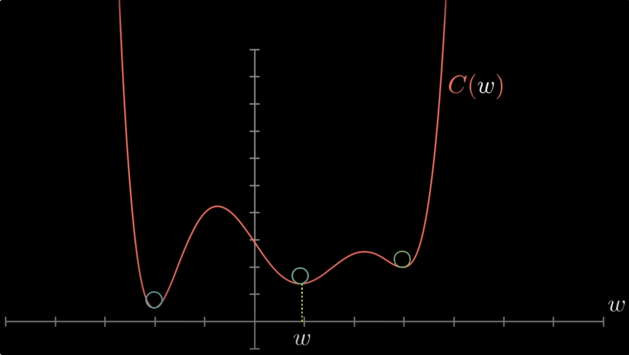
• Local minima. The algorithm follows the slope downhill from wherever you started, which might be into a local basin that isn’t the global optimum. In high dimensions we have no way of knowing whether we’ve found the global minimum.

• Learning rate sensitivity. Too small → painfully slow; too large → oscillation or divergence. See learning-rate.
• Ravines and saddle points. Vanilla GD oscillates across narrow valleys and stalls on flat plateaus. Momentum and Adam (see gradient-descent-variants) address this.

When to stop

Two common criteria:

1. Convergence — loss stops improving over successive iterations.
2. Max iterations — a hyperparameter cap (e.g. 100 epochs). Used in practice because complex models may never fully converge in a reasonable time.

Related

• loss-function — the thing gradient descent minimises
• learning-rate — the step size $\eta$
• gradient-descent-variants — SGD, mini-batch, momentum, Adam
• sigmoid function — the differentiable replacement for sign in classification
• binary-cross-entropy — the classification loss that replaces squared error

Active Recall

Write down the gradient descent update rule and name every symbol.

${\mathbf{\theta }}^{t+1}={\mathbf{\theta }}^t-\eta \nabla L_t$. ${\mathbf{\theta }}^t$ is the current parameter vector, $\nabla L_t$ is the gradient of the loss at those parameters, $\eta$ is the learning rate (step size), and the minus sign flips the uphill gradient into a downhill move.

Why do we subtract the gradient rather than add it?

The gradient points in the direction of steepest increase of the loss. We want to decrease the loss, so we step in the opposite direction. Subtracting is a sign flip that converts ascent into descent.

With ${\hat{x}}^t=21.5$, measurements $\{19,17,24\}$, and loss $L={\sum }_i|x_i-\hat{x}|$, compute the gradient and the next estimate (with $\eta =1$).

Each term contributes $+1$ if $\hat{x}>x_i$ and $-1$ otherwise. Here $21.5>19$ gives $+1$, $21.5>17$ gives $+1$, $21.5<24$ gives $-1$. Sum: $1+1-1=1$. Next estimate: $21.5-1\cdot 1=20.5$.

Why does the gradient descent algorithm fail when the perceptron uses the sign activation with squared loss?

The sign function has derivative zero everywhere it’s defined (and is undefined at zero). By chain rule, $\nabla L$ contains that zero factor, so $\nabla L=0$ identically. The update becomes ${\mathbf{\theta }}^{t+1}={\mathbf{\theta }}^t$ — the parameters never change, and learning is impossible. The fix is to swap sign for a differentiable activation (e.g. sigmoid).

You run gradient descent and the loss jumps up and down between iterations instead of decreasing. What's the likely cause and remedy?

The learning rate is too large — each step overshoots the minimum and lands further from it than before, bouncing around. Reduce $\eta$ (e.g. from 1 to 0.1 or 0.01). You can also use a learning-rate schedule that decays $\eta$ over time.

Why the gradient — what makes it the right direction for descent, rather than just any downhill direction?

From multivariable calculus: among all possible unit directions you could step from your current point, $\nabla L$ is provably the one in which $L$ increases fastest. Its length $\Vert \nabla L\Vert$ is the rate of change in that steepest direction. Negating gives the direction of steepest descent — the single best choice for a local minimisation move.

Give a non-spatial reading of the negative gradient as a prescription over parameters.

Think of $-\nabla L$ as a list of instructions, one per parameter. Each component has a sign (nudge this weight up or down) and a magnitude (how much it matters — a large magnitude means changing this weight will move the loss a lot, a tiny one means it barely matters right now). The gradient thereby encodes the relative importance of every weight and bias — which ones give the best bang for your buck at the current state of training.

Why does gradient descent with a smooth loss (like squared error) tend to settle near a minimum even at a fixed learning rate, whereas with absolute error it oscillates?

For smooth losses the gradient magnitude shrinks continuously as you approach the minimum — the slope flattens — so the step size $\eta \Vert \nabla L\Vert$ also shrinks, and the optimiser decelerates automatically. Absolute error has a kink at the minimum: the gradient magnitude stays at $\pm 1$ right up to the kink, so the step size doesn’t shrink and the iterate leaps back and forth across the minimum instead of closing in.

Gradient descent in 2D lands you in a valley with loss 0.3, but there's a deeper valley elsewhere on the surface with loss 0.05. What happened, and can vanilla gradient descent fix it?

You’ve converged to a local minimum, not the global minimum. Vanilla GD follows the slope downhill from the initialisation, so it can’t climb out of a basin once inside. Remedies: random re-initialisation, momentum (which carries you through shallow basins), or stochastic variants (whose noise can knock you out of local minima).