pooling

Pooling is the cheap, non-learnable counterpart to convolution. It slides a small window over a feature map and reduces each window to a single value — usually the max. The point is to discard spatial precision deliberately, gaining efficiency and shift invariance.

What it does

Like convolution, pooling slides a window over a feature map. Unlike convolution, the operation inside the window is not a dot product — it’s just a fixed function of the window’s values:

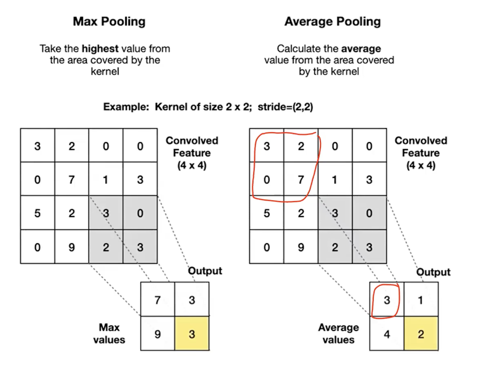
• Max pooling: output the largest value in the window.
• Average pooling: output the mean of the window’s values.

Default settings: window size $F=2$, stride $S=2$. Each output covers a non-overlapping $2\times 2$ patch of the input, so the spatial dimensions are halved. No padding is typical.

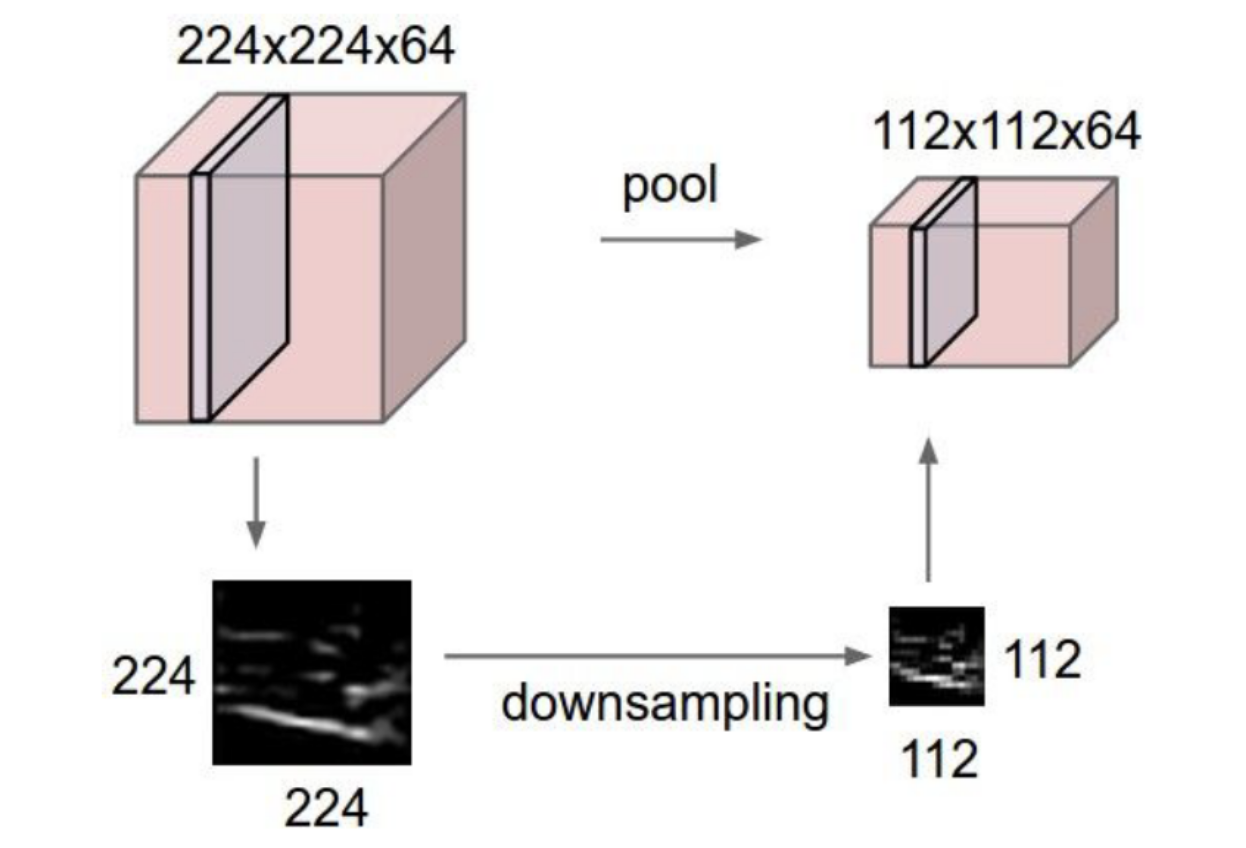
Visually: a $224\times 224\times 64$ feature map becomes $112\times 112\times 64$ — width and height halved, depth untouched. The accompanying greyscale image makes the effect plain: a coarser version of the same content, with fine spatial detail thrown away.

Pooling has zero learnable parameters. It’s a fixed function — not a transformation the network learns. Backpropagation passes gradients through it (with simple rules), but the operation itself is hard-coded.

Pooling operates per-channel

For a feature map of shape $H\times W\times D$, pooling is applied independently to each of the $D$ channels. So an input $H\times W\times D$ becomes $(H/2)\times (W/2)\times D$ after a $2\times 2$ pool with stride 2 — depth is preserved, only spatial dimensions shrink.

This matters: convolution mixes channels (each filter touches every input channel); pooling never mixes channels. So a CNN’s depth dimension is built up by convolution alone.

Output size formula

Same shape as the convolution magic formula, but with no padding (typical) and depth unchanged:

$W_2=\frac{W_1-F}{S}+1,H_2=\frac{H_1-F}{S}+1,D_2=D_1$

For the canonical $F=2,S=2$:

$W_2=\frac{W_1-2}{2}+1=\frac{W_1}{2}$

(when $W_1$ is even, which it usually is by design).

Max vs average — when each makes sense

	Max pooling	Average pooling
What it preserves	The strongest activation in the region	The general level across the region
Loss of info	Discards everything but the max	Smears the region’s information together
Common use	Interior of CNNs (the default)	Final pooling before classification (global average pooling)

Max pooling fits the feature-extraction story well: a high activation means “this filter detected its feature here”. The maximum tells you whether the feature was detected anywhere in the region; the exact location within the region is intentionally discarded. That’s the shift-invariance contribution — see shift-invariance-equivariance.

Average pooling smooths instead of selecting. Global average pooling (window size = whole feature map) is sometimes used at the end of a CNN as an alternative to flatten + FC: average each channel into a single value, giving a $D$-dim vector for classification. It has fewer parameters than the equivalent FC head.

Worked example

Take a $4\times 4$ feature map (single channel, for clarity):

$\left(\begin{array}{cccc}1& 1& 2& 4\\ 5& 6& 7& 8\\ 3& 2& 1& 0\\ 1& 2& 3& 4\end{array}\right)$

Apply $2\times 2$ max pooling, stride 2. Four non-overlapping $2\times 2$ regions, output is $2\times 2$:

$\left(\begin{array}{cc}\max (1,1,5,6)& \max (2,4,7,8)\\ \max (3,2,1,2)& \max (1,0,3,4)\end{array}\right)=\left(\begin{array}{cc}6& 8\\ 3& 4\end{array}\right)$

With average pooling on the same input, the values would be 3.25, 5.25, 2, 2.

Why pooling helps

1. Compute and memory savings. Halving spatial dimensions cuts the activation count by $4\times$ (in 2D). A network that keeps full resolution through 10 conv layers would have impractical memory cost; periodic pooling makes deep networks feasible.

2. Shift invariance. If a feature shifts by 1 pixel within a $2\times 2$ region, the max value is unchanged. Stack several pool layers and the network becomes insensitive to small spatial shifts of the input — which is what you want for “this is a cat, regardless of where in the frame it sits”. See shift-invariance-equivariance for the full story.

3. Implicit hierarchy of receptive fields. Each pool layer doubles the effective receptive field of subsequent conv layers. Early layers see small windows (edges, dots); after pooling, deeper layers see proportionally larger windows of the original image (shapes, parts, objects). Pooling is a key way the network builds the low → mid → high feature hierarchy.

When not to pool

For tasks that need to predict at full input resolution — like semantic segmentation (label every pixel) — pooling is undesirable because it throws away the spatial precision the output needs. Fully convolutional networks (FCNs) for segmentation either skip pooling entirely (preserves resolution but expensive) or do downsample-then-upsample (encoder-decoder) to keep compute manageable while reconstructing per-pixel output.

The general lesson: pooling is an opinion about what to lose. For classification, losing precise location is helpful. For segmentation, it’s a problem to be undone.

Backprop through pooling

Although pooling has no parameters, it’s part of the forward pass and must propagate gradients backward:

• Max pooling: the gradient is routed only to the position that contained the max. All other positions in the window receive zero gradient. (Implementations cache the index of the max during the forward pass.)
• Average pooling: the gradient is split equally across every position in the window — each gets $1/F^2$ of the upstream gradient.

In both cases, the backward pass is fast and parameter-free. See backpropagation for the broader principle of routing gradients backward through every operation.

Pooling vs strided convolution

A convolution with stride 2 also halves spatial size — and unlike pooling, it has learnable parameters. Some modern architectures (like ResNet’s transition layers) use strided convolution in place of pooling. Trade-offs:

• Strided conv: Learnable. Can extract features and downsample in one operation. More parameters.
• Pooling: Free. Hard-codes the downsampling rule (max or average). No flexibility.

Both are still in widespread use; pooling persists because it’s cheap and well-understood.

Related

• convolution — the other half of the conv-pool block; pooling typically follows convolution + activation
• convolutional-neural-network — the architecture where pooling sits between convolutional blocks
• shift-invariance-equivariance — pooling is the architectural source of shift invariance
• backpropagation — even though pooling has no parameters, gradients flow through it (via the max-index or average rule)

Active Recall

What is the output of a $2\times 2$ max pooling with stride 2 applied to the $4\times 4$ matrix $\left(\begin{array}{cccc}1& 2& 3& 4\\ 5& 6& 7& 8\\ 9& 1& 2& 3\\ 4& 5& 6& 7\end{array}\right)$?

Four non-overlapping $2\times 2$ regions: $\max (1,2,5,6)=6$, $\max (3,4,7,8)=8$, $\max (9,1,4,5)=9$, $\max (2,3,6,7)=7$. Output: $\left(\begin{array}{cc}6& 8\\ 9& 7\end{array}\right)$.

A $112\times 112\times 64$ feature map is processed by $2\times 2$ max pooling with stride 2. What's the output shape, and how many learnable parameters does this layer add?

Output spatial size: $(112-2)/2+1=56$, so $56\times 56$. Depth is unchanged at 64. Output shape: $56\times 56\times 64$. Learnable parameters: zero — pooling has no weights or biases.

Why is max pooling typically preferred over average pooling in the interior of a CNN?

Each value in a feature map is the activation of a feature detector — high values mean “this feature was found here”. The maximum within a window says “the feature was found somewhere in this region”, which is exactly what feature extraction wants to preserve. Averaging dilutes that signal: a strong response in one position gets blurred with weak responses elsewhere. For the deeper layers’ purpose (knowing whether features exist, not exactly where), max is the cleaner summary.

How does pooling contribute to shift invariance, and why does that help classification?

If a feature shifts by 1–2 pixels within a pooling window, the max value (and roughly the average) doesn’t change — the post-pool output is the same. So the network’s deeper layers receive the same input regardless of small spatial shifts. After several pool layers compounded with downstream FC layers (which don’t preserve spatial position at all), the final classification is unaffected by where in the image the object sat. For classification — “is this a cat?” — that’s exactly the right invariance.

For a CNN doing semantic segmentation (label every pixel), why is pooling problematic, and how do networks like FCN handle it?

Pooling discards spatial precision: a $2\times 2$ max-pool says “feature was in this region” without saying where in the region. That’s fatal for per-pixel prediction. FCN-style networks either avoid pooling (and pay the compute cost of full-resolution feature maps throughout) or use an encoder-decoder structure: downsample for efficient feature extraction, then upsample (transpose convolution, etc.) back to the original resolution before predicting. The U-Net architecture (week 5) is a popular encoder-decoder design for segmentation.

During backpropagation, how do gradients flow through max pooling vs average pooling?

Max pooling: the gradient at the pooled output is routed only to the input position that contained the max during the forward pass. Other positions in the window receive zero gradient. (Hence implementations cache the max-index.) Average pooling: the gradient at the output is divided equally among all positions in the window — each gets $1/F^2$ of the upstream gradient. Either way the operation has no parameters; backprop just routes gradients to upstream activations.