backpropagation

The algorithm that makes training deep networks tractable. Gradient descent answers “what do we do with $\nabla L$?”; backpropagation answers “how do we compute $\nabla L$ efficiently, for every parameter, in a network with millions of them?”

What problem it solves

gradient descent needs $\nabla L$ to update weights. For a single perceptron, computing each $\partial L/\partial w_i$ by hand is easy. For an MLP with three hidden layers and 36 weights, it’s tedious. For a real network with millions or billions of parameters, naive derivative computation would be:

• Too hard by hand — you can’t plausibly write down a closed-form expression for every parameter’s gradient.
• Computationally wasteful — many intermediate derivatives (e.g. $\partial L/\partial z_1^2$) appear inside the chain-rule expressions for multiple parameters. Recomputing them is redundant.

Backpropagation solves both at once. It walks the computation-graph representing the network and computes all parameter gradients in two passes.

Intuition: what does a single training example want?

Before the math, here’s the framing that makes backprop click. Take an MLP trained to classify MNIST digits. Show it a hand-drawn “2”. The network’s output layer is 10 neurons (one per digit). At first, the output activations are random — say $(0.5,0.8,0.2,1.0,0.4,0.6,1.0,0.0,0.2,0.1)$.

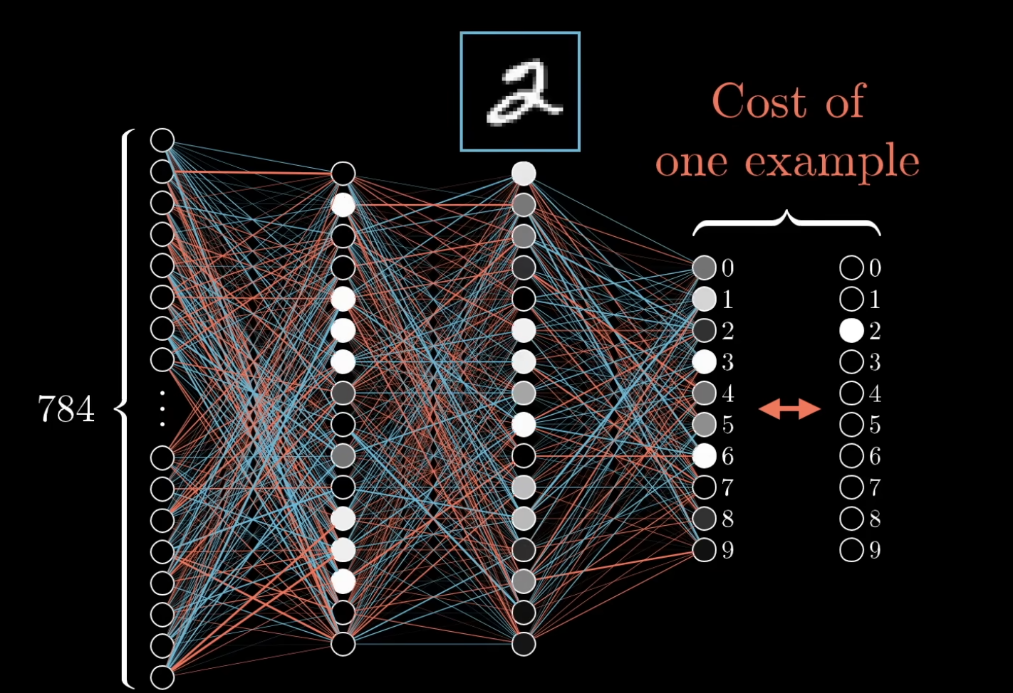
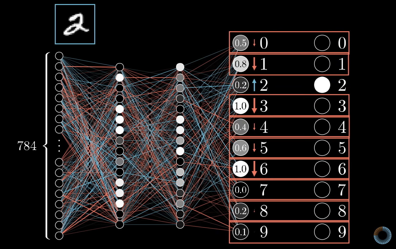
We want the “2” neuron to be high and every other neuron to be low. Each output neuron needs a nudge:

• “2” neuron at 0.2 → nudge up, by a lot.
• “3” neuron at 1.0 → nudge down, by a lot.
• “7” neuron at 0.0 → already low, nudge down only a little.

The size of each nudge is proportional to how far the current activation is from where it should be. Confidently-wrong activations need the biggest pushes; nearly-right ones barely need touching.

Three avenues to nudge a neuron’s activation

We can’t change activations directly — we can only change weights and biases. For a single output neuron with activation $a=\sigma ({\sum }_i{w}_i{a}_i+b)$, there are three knobs:

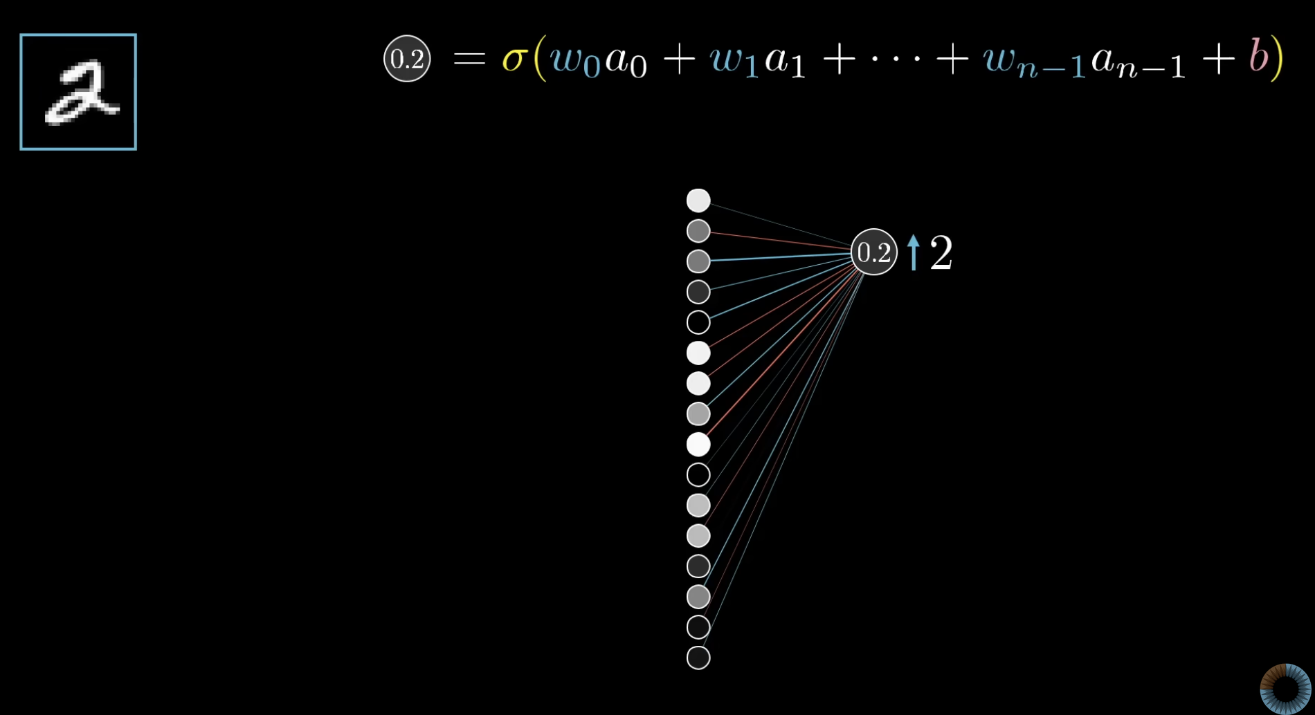
1. Increase the bias $b$ — a uniform additive nudge to $z$, which pushes $a$ up.
2. Increase the weights $w_i$ in proportion to the incoming activations $a_i$ — incoming connections from brighter (more active) previous-layer neurons have bigger leverage on $z$, so changing those weights gives more bang for the buck. Connections from dim neurons barely matter.
3. Change the activations $a_i$ from the previous layer in proportion to $w_i$ — we can’t directly modify $a_i$ (those are decided by even-earlier weights), but we can record what we wish $a_i$ would do, and propagate that wish backward.

Notice that avenues 2 and 3 are mirror images of each other. Both depend on the product $w_i\cdot a_i$. The connections that matter most are those between active neurons and high-leverage weights.

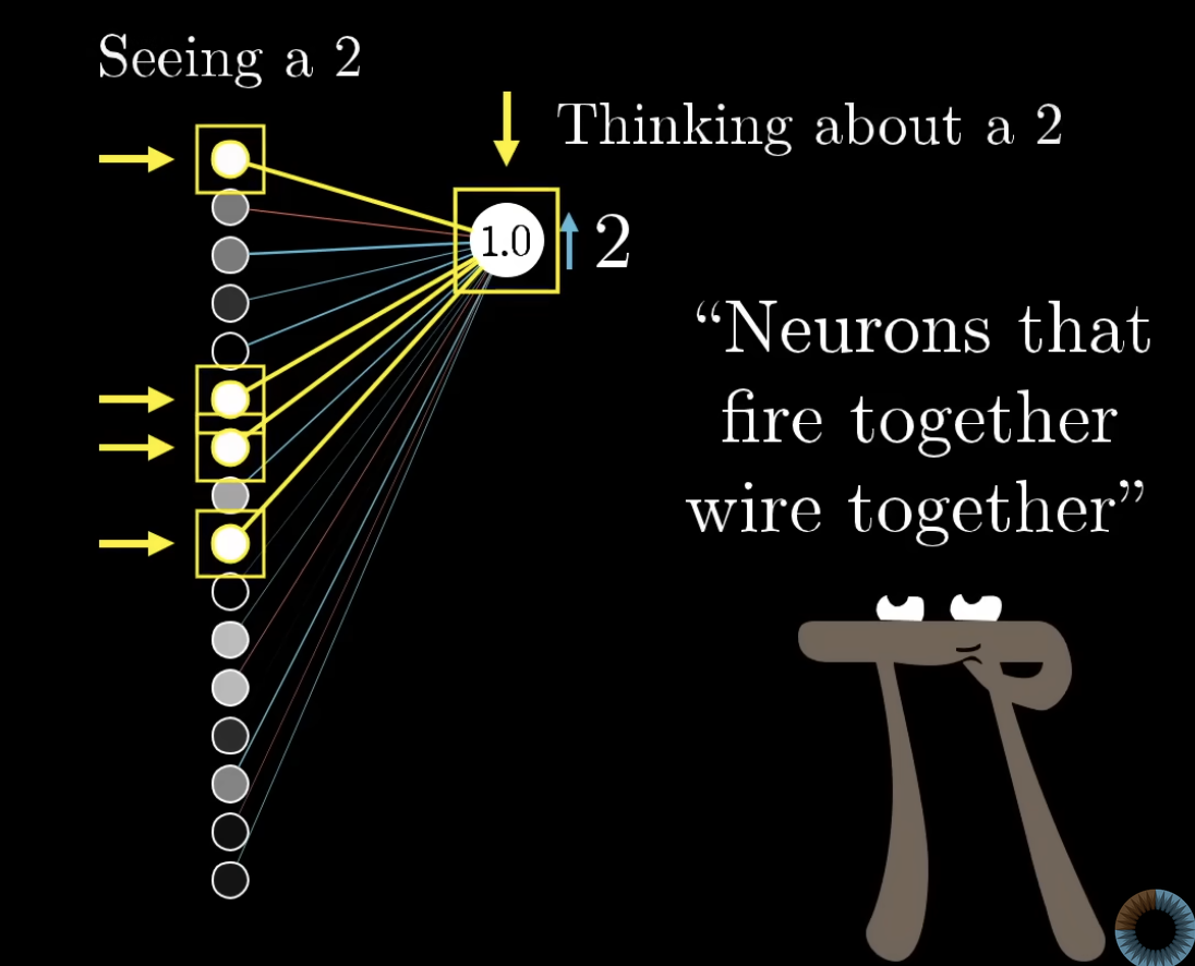
TIP — "Neurons that fire together, wire together"

Avenue 2 says weights from active neurons get strengthened. This mirrors Hebbian theory in neuroscience: when two neurons co-activate during learning, the connection between them strengthens. The biological brain learns roughly the same way an MLP does — by reinforcing connections between neurons that are active when the desired output occurs.

Recursing backward through the network

For each output neuron, we now have a list of desired changes for the previous layer’s activations (avenue 3). But every output neuron has its own list — they each have opinions on what the previous layer should do. Sum these opinions across all output neurons (weighted by the corresponding $w_i$ and by how much each output neuron itself wanted to change). The result: a single list of desired nudges to the previous layer.

That list now becomes the new “what we want” for the previous layer, and we repeat the whole argument one layer further back: this layer’s desires get translated into desired weight/bias changes within it, plus desired activation changes for its previous layer, which we then propagate again.

This is backpropagation. We start at the output, decide what each neuron wants, translate that into local weight/bias updates, and recursively pass the resulting “desires” backward through the network until every parameter has its update.

Averaging across training examples

The above is what one training example wants. If you only used one example, the network would just learn to classify everything as that example’s class. To get a real gradient, run backprop for every training example, record each example’s desired changes, and average them.

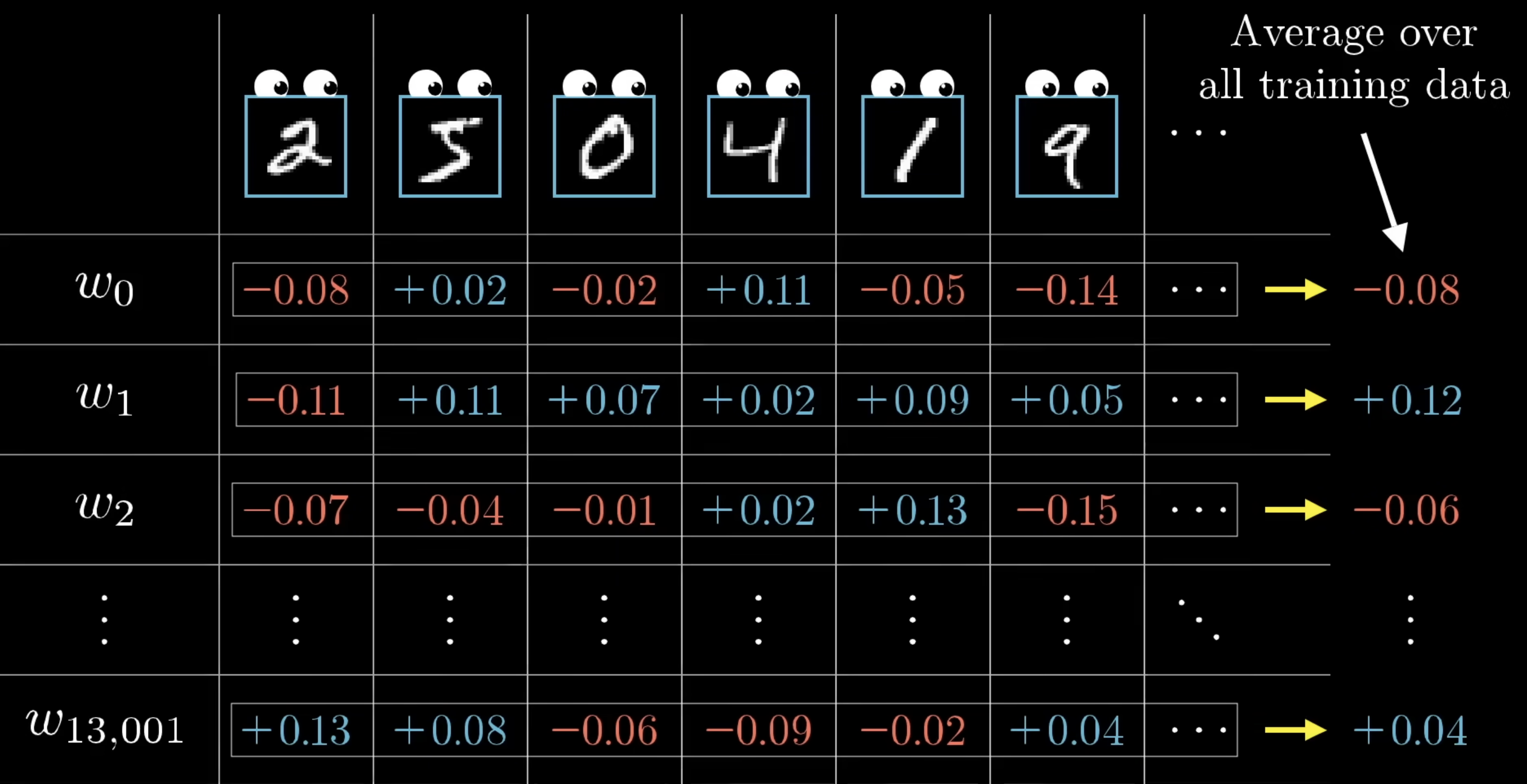
That averaged list of desired changes is — up to a sign — exactly the negative gradient $-\nabla L$ of the cost function. Backpropagation is how we compute this gradient; gradient descent is what uses it.

In practice, averaging over the full training set per step is too slow, so we use mini-batch SGD: average over a random subset of examples, take a step, repeat with a new subset. The gradient estimates are noisier but training is much faster.

What the gradient magnitudes mean

The component of $-\nabla L$ for a particular weight tells you how sensitive the cost is to that weight. If one component is 32 times larger than another, the cost is 32 times more sensitive to changes in the first weight. Backprop doesn’t just tell you “nudge each weight up or down” — it tells you which weights give the most cost reduction per unit of nudging. That’s why gradient descent works as well as it does (see also the non-spatial reading of the gradient in gradient descent).

The mathematical foundation: chain rule

Univariate chain rule

If $f=f(g)$ and $g=g(t)$, then:

$\frac{\partial f}{\partial t}=\frac{\partial f}{\partial g}\cdot \frac{\partial g}{\partial t}$

Picture: $t\to g\to f$. The sensitivity of $f$ to $t$ is the product of the two links in the chain.

Multivariate chain rule

If $f$ depends on multiple intermediates that all trace back to $t$ — formally $f=f(g_1,\dots ,g_n)$ with each $g_i=g_i(t)$ — then the chain rule sums contributions from every path:

$\frac{\partial f}{\partial t}={\sum }_{i=1}^n\frac{\partial f}{\partial g_i}\cdot \frac{\partial g_i}{\partial t}$

Picture: $t$ fans out to $g_1,\dots ,g_n$, which converge back to $f$. The sensitivity of $f$ to $t$ accumulates across all paths.

TIP — Why the multivariate case matters for networks

A single weight early in a network often influences many downstream neurons, so the output depends on it through multiple paths. The multivariate chain rule says: to get the true gradient, sum the contribution from every path. This is exactly what backpropagation does automatically.

Chain rule in a computation graph

Generalising to any computation-graph node $t$ with successors $g_1,\dots ,g_n$ (the nodes $t$ flows into):

$\frac{\partial f}{\partial t}={\sum }_{i:g_i\text{ is a successor of }t}\frac{\partial f}{\partial g_i}\cdot \frac{\partial g_i}{\partial t}$

The gradient at a node is built from the gradients at its successors. This is the key recursion that backpropagation exploits.

Applying the chain rule to a single neuron’s weight

Concretely, for a weight $w^{(L)}$ feeding into the final layer of an MLP, the cost flows through this chain:

$w^{(L)}⟶z^{(L)}⟶a^{(L)}⟶C$

with

• $z^{(L)}=w^{(L)}{a}^{(L-1)}+b^{(L)}$ — the weighted sum
• $a^{(L)}=\sigma (z^{(L)})$ — the activation
• $C=(a^{(L)}-y{)}^2$ — the cost (squared error here)

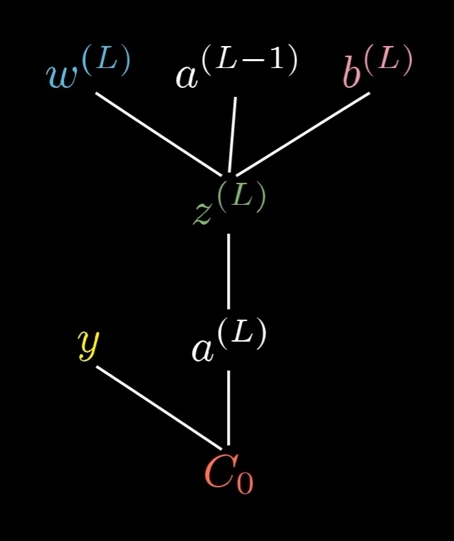
The cost $C$ depends on $w^{(L)}$, $a^{(L-1)}$, and $b^{(L)}$ all through the same intermediate $z^{(L)}$ — and through one more activation step $a^{(L)}=\sigma (z^{(L)})$ before reaching $C$.

The chain rule decomposes the gradient into three meaningful pieces:

$\frac{\partial C}{\partial w^{(L)}}=\underset{\text{output-vs-target}}{\underbrace{\frac{\partial C}{\partial a^{(L)}}}}\cdot \underset{\text{activation slope}}{\underbrace{\frac{\partial a^{(L)}}{\partial z^{(L)}}}}\cdot \underset{\text{previous activation}}{\underbrace{\frac{\partial z^{(L)}}{\partial w^{(L)}}}}$

Read it as a sequence of three nudges: a tiny change in $w^{(L)}$ produces a small change in $z^{(L)}$, which produces a small change in $a^{(L)}$, which produces a small change in $C$. Multiply the three sensitivities and you get the total sensitivity of $C$ to $w^{(L)}$.

Each piece has a clear interpretation:

• $\partial C/\partial a^{(L)}=2(a^{(L)}-y)$ — proportional to how wrong the network is. Big error → big gradient signal.
• $\partial a^{(L)}/\partial z^{(L)}={\sigma }^{\prime }(z^{(L)})$ — the slope of the activation function at the current pre-activation. If $\sigma$ is saturated, this is near zero and the gradient vanishes (a hint of why deep networks have trouble — see future weeks).
• $\partial z^{(L)}/\partial w^{(L)}=a^{(L-1)}$ — the activation of the previous neuron. Brighter (more active) previous neurons mean bigger gradient, which is exactly the “fire together, wire together” intuition formalised.

Multiply them together and you have the gradient for one weight. The same recipe applies to every weight in the network — you just chain through more layers.

The bias gradient

Same chain, different last factor. For the bias $b^{(L)}$:

$\frac{\partial C}{\partial b^{(L)}}=\frac{\partial C}{\partial a^{(L)}}\cdot \frac{\partial a^{(L)}}{\partial z^{(L)}}\cdot \frac{\partial z^{(L)}}{\partial b^{(L)}}=2(a^{(L)}-y)\cdot {\sigma }^{\prime }(z^{(L)})\cdot 1$

The first two factors are identical to the weight gradient. Only the last one differs: $\partial z^{(L)}/\partial b^{(L)}=1$ (because $b$ enters $z$ additively without a multiplier). So $\partial C/\partial b^{(L)}$ is just $\partial C/\partial w^{(L)}$ with the $a^{(L-1)}$ factor stripped out.

The “previous activation” gradient — and the symmetry that makes recursion natural

To recurse one layer back, we need $\partial C/\partial a^{(L-1)}$ — the cost’s sensitivity to the previous layer’s output. Same chain again:

$\frac{\partial C}{\partial a^{(L-1)}}=\frac{\partial C}{\partial a^{(L)}}\cdot \frac{\partial a^{(L)}}{\partial z^{(L)}}\cdot \frac{\partial z^{(L)}}{\partial a^{(L-1)}}=2(a^{(L)}-y)\cdot {\sigma }^{\prime }(z^{(L)})\cdot w^{(L)}$

Compare the weight gradient and the previous-activation gradient side by side:

$\frac{\partial C}{\partial w^{(L)}}=2(a^{(L)}-y)\cdot {\sigma }^{\prime }(z^{(L)})\cdot \boxed{a^{(L-1)}}$ $\frac{\partial C}{\partial a^{(L-1)}}=2(a^{(L)}-y)\cdot {\sigma }^{\prime }(z^{(L)})\cdot \boxed{w^{(L)}}$

The two formulas are identical except for the last factor — and the swap is between $w^{(L)}$ and $a^{(L-1)}$. This symmetry comes from $z^{(L)}=w^{(L)}{a}^{(L-1)}+b^{(L)}$ being symmetric in $w$ and $a^{(L-1)}$ (each is the other’s coefficient). It’s the same principle as Hebbian “fire together, wire together” — the importance of the connection $w\cdot a^{(L-1)}$ depends on both of them — but now seen from the other side: when you ask how much the cost depends on $a^{(L-1)}$, the answer is weighted by $w$ exactly as how-much-it-depends-on-$w$ was weighted by $a^{(L-1)}$.

Once $\partial C/\partial a^{(L-1)}$ is known, treat $a^{(L-1)}$ as the “output” of layer $L-1$ and apply the same three-factor recipe to compute $\partial C/\partial w^{(L-1)}$, $\partial C/\partial b^{(L-1)}$, and $\partial C/\partial a^{(L-2)}$. Iterate. Backpropagation is just this same chain rule, applied recursively backwards through the layers.

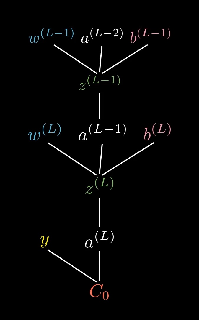
The dependency tree literally extends one layer up: $w^{(L-1)},a^{(L-2)},b^{(L-1)}\to z^{(L-1)}\to a^{(L-1)}$, and now $a^{(L-1)}$ is just an input to the same downstream chain we already analysed. The structure is self-similar — every layer looks like every other layer, only with shifted indices.

All four gradients in one place (one-neuron-per-layer case)

For the simplest network — one neuron per layer, squared-error loss, sigmoid activation, illustrated above as a chain of four neurons (the colour gradient suggests increasing activation from left to right) — all the gradients you ever need are these:

$\frac{\partial C}{\partial w^{(L)}}=a^{(L-1)}\cdot {\sigma }^{\prime }(z^{(L)})\cdot 2(a^{(L)}-y)$ $\frac{\partial C}{\partial b^{(L)}}=1\cdot {\sigma }^{\prime }(z^{(L)})\cdot 2(a^{(L)}-y)$ $\frac{\partial C}{\partial a^{(L-1)}}=w^{(L)}\cdot {\sigma }^{\prime }(z^{(L)})\cdot 2(a^{(L)}-y)$

Then recurse: replace $L$ with $L-1$, replace $2(a^{(L)}-y)$ with the just-computed $\partial C/\partial a^{(L-1)}$, and repeat. Every gradient in the entire network is some chain of these three patterns.

Multi-path version for hidden activations

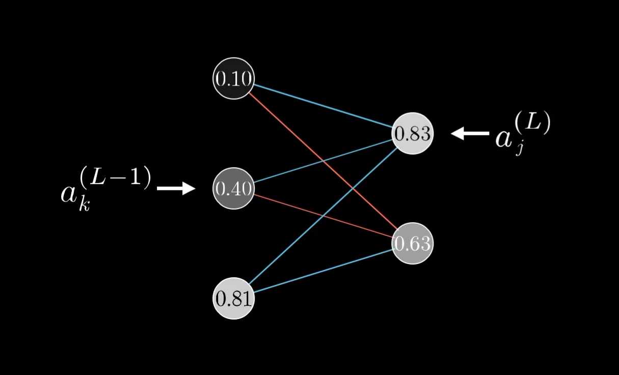
For a hidden activation $a_k^{(L-1)}$ in layer $L-1$, the cost depends on it through every neuron in layer $L$. Apply the multivariate chain rule:

$\frac{\partial C}{\partial a_k^{(L-1)}}={\sum }_j\frac{\partial C}{\partial a_j^{(L)}}\cdot \frac{\partial a_j^{(L)}}{\partial z_j^{(L)}}\cdot \frac{\partial z_j^{(L)}}{\partial a_k^{(L-1)}}$

Each term in the sum is one path from $a_k^{(L-1)}$ to $C$ through one of the next-layer neurons. The “desires” of all next-layer neurons get added up — exactly as the intuition section described.

Once $\partial C/\partial a_k^{(L-1)}$ is known, the same chain-rule trick extends backward to compute $\partial C/\partial w^{(L-1)}$ and $\partial C/\partial b^{(L-1)}$, and so on through every earlier layer. Backpropagation is just this iteration: solve the layer you’re on using gradients from the layer ahead, then move one layer back.

TIP — Multi-neuron layers don't add new ideas, just bookkeeping

The one-neuron-per-layer case has all the conceptual content of backpropagation. When layers are wider:

• Each weight $w_{jk}^{\ell }$ still gets a three-factor gradient — same formula, just decorated with $j$ and $k$ indices.
• Each previous-layer activation $a_k^{(L-1)}$ now influences the cost through every next-layer neuron $j$, so its gradient becomes a sum across $j$ — that’s the multivariate chain rule from earlier.
• In matrix form, the sums become matrix multiplications and the whole layer’s gradients fit on one line. Implementations use vector/matrix operations to hide the indices.

What does not change: the chain rule, the three pieces, the symmetry between weight and previous-activation gradients, or the recursive backward pass. If you understand the simplest case, you understand backprop. The rest is implementation detail.

The matrix-form summary captures this — the same three-factor pattern, decorated with sums across $j$ in the multi-neuron case, and recursively applying $\partial C/\partial a^{(\ell +1)}$ to compute $\partial C/\partial a^{(\ell )}$:

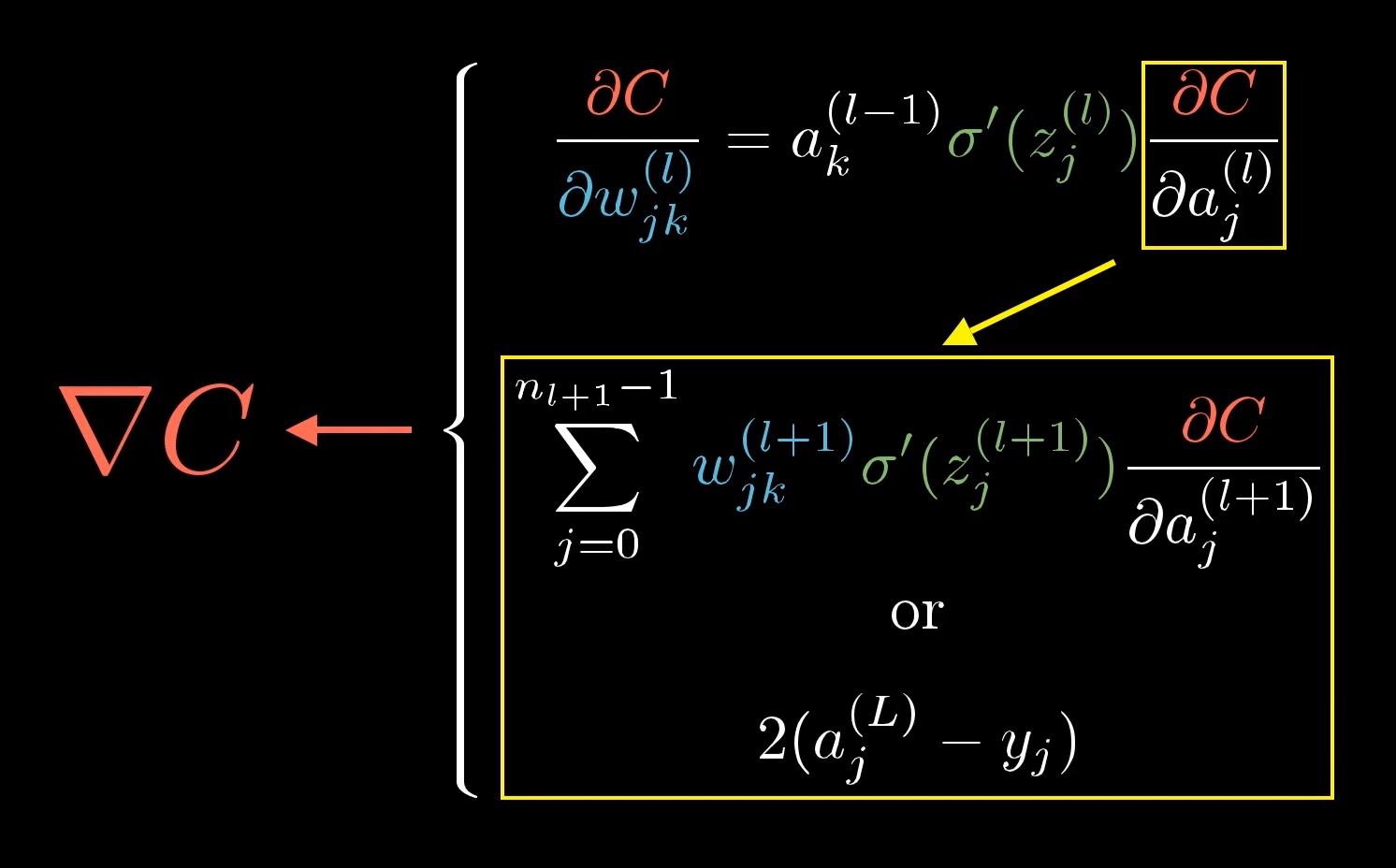
The boxed term on the right (in 3B1B’s diagram) is the recursion: $\partial C/\partial a_j^{(L)}$ at the output layer is just $2(a_j^{(L)}-y_j)$ from the squared-error loss, and at every other layer it’s a sum across the layer ahead — exactly the multivariate chain rule expressed in indexed form.

The algorithm: forward pass + backward pass

Forward pass

Walk the computation graph from inputs to output. At each node, compute its value from its predecessors’ values and cache it. By the end, you have:

• The output / loss at the final node.
• All intermediate values stored at every node in between.

The forward pass does exactly what inference does — it’s just evaluating the network.

Backward pass

Walk the graph from the output back to the inputs. At each node $t$, compute $\partial L/\partial t$ using the chain rule:

$\frac{\partial L}{\partial t}={\sum }_{i:g_i\text{ is a successor of }t}\frac{\partial L}{\partial g_i}\cdot \frac{\partial g_i}{\partial t}$

Because we walk backwards, the gradients $\partial L/\partial g_i$ at each successor are already computed by the time we visit $t$. We just multiply by the local derivative $\partial g_i/\partial t$ (which uses cached forward-pass values) and sum.

By the end of the backward pass, every parameter node has its gradient $\partial L/\partial w$, ready to feed into the gradient-descent update.

Worked example: $z=(a+b)(b+c)$

Take $a=-1$, $b=3$, $c=4$.

Forward pass

Node	Computation	Value
$a$	—	$-1$
$b$	—	$3$
$c$	—	$4$
$x$	$a+b$	$2$
$y$	$b+c$	$7$
$z$	$x\cdot y$	$14$

Backward pass

Start from the output. $\partial z/\partial z=1$ trivially. Move backwards:

Target	Using	Calculation	Value
$\partial z/\partial x$	$z=xy$, so $\partial z/\partial x=y$	$y=7$	$7$
$\partial z/\partial y$	$z=xy$, so $\partial z/\partial y=x$	$x=2$	$2$
$\partial z/\partial a$	$\partial z/\partial x\cdot \partial x/\partial a$	$7\cdot 1$	$7$
$\partial z/\partial c$	$\partial z/\partial y\cdot \partial y/\partial c$	$2\cdot 1$	$2$
$\partial z/\partial b$	Two paths: $b\to x\to z$ and $b\to y\to z$. Multivariate chain rule: $\partial z/\partial x\cdot \partial x/\partial b+\partial z/\partial y\cdot \partial y/\partial b$	$7\cdot 1+2\cdot 1$	$9$

Every partial derivative $\partial z/\partial g_i$ was computed once and reused for each predecessor. That’s the efficiency win.

A second example with a non-linear node: $z=a^2(a+b)$

This time $a$ feeds into two downstream paths (the squaring node and the addition node), so even though the graph looks small, the multivariate chain rule applies.

Graph: $a,b$ are inputs; $x=a^2$ via the squaring node; $y=a+b$ via the addition node; $z=x\cdot y$ at the output.

For $a=1,b=-2$:

Forward: $x=1^2=1$, $y=1+(-2)=-1$, $z=1\cdot (-1)=-1$.

Backward:

• $\partial z/\partial x=y=-1$
• $\partial z/\partial y=x=1$
• $\partial z/\partial a$ — two paths, sum them: $\frac{\partial z}{\partial a}=\frac{\partial z}{\partial x}\frac{\partial x}{\partial a}+\frac{\partial z}{\partial y}\frac{\partial y}{\partial a}=(-1)(2a)+(1)(1)=-2+1=-1$
• $\partial z/\partial b=(\partial z/\partial y)(\partial y/\partial b)=1\cdot 1=1$

The pattern is identical to the previous example — only difference is one of the local derivatives ($\partial x/\partial a=2a$) involves a forward-pass value, which is why caching forward values matters.

Why “backward”? Why not compute everything forward?

You could compute gradients forward — it’s called forward-mode automatic differentiation, and for each parameter it propagates $\partial (\cdot )/\partial w$ alongside the forward values. But forward mode computes the gradient with respect to one input at a time. For a network with $N$ parameters, you’d need $N$ forward passes to get every gradient.

Backward mode (backprop) computes the gradient with respect to one output at a time — and a neural network has one scalar loss output. A single backward pass gets you all $N$ parameter gradients. For deep networks with huge $N$ and a single loss, backward mode is asymptotically cheaper. That’s why everyone uses it.

Connection to gradient descent

Backpropagation produces $\nabla L$. Plug it into the gradient descent update:

${\mathbf{\theta }}^{t+1}={\mathbf{\theta }}^t-\eta \nabla L_t$

and the weights move a small step downhill. Repeat: forward pass → backward pass → update → forward pass → … until convergence (or until you hit the epoch budget). This loop — forward, backward, update — is the training loop for essentially every modern neural network.

One useful framing: at inference time (predicting on new inputs), you only run the forward pass. The backward pass is training-only infrastructure. Once training finishes, you throw away the gradient machinery and keep the learned weights.

Efficiency: the reuse principle

The key insight is that the same intermediate gradients appear in many parameter gradients. In $z=(a+b)(b+c)$:

• $\partial z/\partial x$ is used to compute both $\partial z/\partial a$ and (part of) $\partial z/\partial b$.
• $\partial z/\partial y$ is used to compute both $\partial z/\partial c$ and (part of) $\partial z/\partial b$.

Compute each intermediate gradient once, cache it at the node, reuse everywhere. This turns a naive $O(\text{paths})$ computation into an efficient $O(\text{nodes})$ one. Without this reuse, training deep networks would be impossible.

Related

• computation-graph — the data structure backprop walks
• gradient descent — the consumer of backprop’s output
• multi-layer-perceptron — the canonical application
• loss-function — the scalar backprop differentiates

Active Recall

What do the forward pass and backward pass each compute, and why does the forward pass happen first?

The forward pass walks the computation graph from inputs to output, computing and caching the value at every intermediate node — ending with the loss at the output. The backward pass then walks backwards, computing $\partial L/\partial t$ at each node by combining gradients from its successors with its local derivative. Forward must happen first because the backward pass uses the cached forward-pass values to evaluate local derivatives (e.g. $\partial (xy)/\partial x=y$ needs the current value of $y$).

Apply the multivariate chain rule: for $z=(a+b)(b+c)$ with $a=0$, $b=2$, $c=5$, compute $\partial z/\partial b$.

Forward: $x=a+b=2$, $y=b+c=7$. Local derivatives: $\partial z/\partial x=y=7$, $\partial z/\partial y=x=2$, $\partial x/\partial b=1$, $\partial y/\partial b=1$. Multivariate chain rule: $\partial z/\partial b=7\cdot 1+2\cdot 1=9$.

Why is backpropagation called backpropagation rather than just "automatic differentiation"?

Because it propagates the error signal (gradient of the loss) backwards through the network, from the output layer to the input layer. Each layer receives the gradient from its successor layer, adjusts it by its local derivative, and passes it to its predecessor. The directionality of this gradient flow — from the loss, back to each parameter — is exactly opposite the forward data flow, hence “back-propagation”.

A weight early in a deep network influences many paths to the output. How does backpropagation handle this correctly without repeated computation?

It uses the multivariate chain rule at every node: $\partial L/\partial t={\sum }_i(\partial L/\partial g_i)(\partial g_i/\partial t)$ where the sum is over all successors $g_i$. Each path’s contribution is accumulated at the node $t$ as a sum. The algorithm computes each $\partial L/\partial g_i$ exactly once (caching it when it visits $g_i$) and reuses it for every predecessor — so the total work is proportional to the number of nodes, not the number of paths.

Why do deep learning practitioners prefer backward-mode over forward-mode automatic differentiation for training neural networks?

Forward mode computes $\partial (\text{everything})/\partial (\text{one input})$ in a single pass — good when you have few inputs and many outputs. Backward mode computes $\partial (\text{one output})/\partial (\text{everything})$ in a single pass — good when you have one output (a scalar loss) and many inputs (millions of parameters). Neural network training is exactly the latter case: one scalar loss, many parameters, so a single backward pass gets every parameter’s gradient. Forward mode would need one pass per parameter.

At inference time (using a trained model to predict), which pass(es) do you actually need?

Only the forward pass. The backward pass is used during training to compute gradients for parameter updates. Once training is complete and the weights are fixed, prediction on a new input just involves running the forward pass to compute the output — no gradients, no weight updates.

Backprop on one training example tells you how that single example wants the weights to change. Why is averaging across the training set crucial, and what does the average correspond to mathematically?

Training on a single example would push the network to classify everything as that example’s class — useless. Averaging the per-example desired changes across the full training set produces a balanced update direction that helps every example a little, rather than one example a lot. Mathematically the average is the negative gradient $-\nabla L$ of the loss (which is itself an average over examples), so per-example backprop + averaging = computing $-\nabla L$. In practice, averaging over mini-batches instead of the full dataset is much faster while still being a good gradient estimate.

Compare $\partial C/\partial w^{(L)}$ and $\partial C/\partial a^{(L-1)}$ for a one-neuron-per-layer network. What's the same, and what's different?

Both are products of three factors $\partial C/\partial a^{(L)}\cdot \partial a^{(L)}/\partial z^{(L)}\cdot (\text{something})$. The first two factors — output error and activation slope — are identical in both. The only difference is the last factor: $\partial z^{(L)}/\partial w^{(L)}=a^{(L-1)}$ for the weight gradient, $\partial z^{(L)}/\partial a^{(L-1)}=w^{(L)}$ for the previous-activation gradient. The weight gradient is weighted by how active the previous neuron was; the previous-activation gradient is weighted by how strong the connecting weight was. The two formulas are symmetric in $w$ and $a^{(L-1)}$, which is why backprop’s recursion feels so clean — the same three-piece pattern works for every gradient.

For a one-neuron-per-layer network with squared error and sigmoid activation, write down $\partial C/\partial w^{(L)}$, $\partial C/\partial b^{(L)}$, and $\partial C/\partial a^{(L-1)}$ in compact form.

$\partial C/\partial w^{(L)}=a^{(L-1)}\cdot {\sigma }^{\prime }(z^{(L)})\cdot 2(a^{(L)}-y)$. $\partial C/\partial b^{(L)}=1\cdot {\sigma }^{\prime }(z^{(L)})\cdot 2(a^{(L)}-y)$ (same as the weight gradient with the $a^{(L-1)}$ factor stripped — because $b$ enters $z$ without a multiplier). $\partial C/\partial a^{(L-1)}=w^{(L)}\cdot {\sigma }^{\prime }(z^{(L)})\cdot 2(a^{(L)}-y)$. The first two factors are shared; only the last one differs based on what we’re differentiating with respect to.

The chain rule decomposition $\partial C/\partial w^{(L)}=(\partial C/\partial a)(\partial a/\partial z)(\partial z/\partial w)$ has three factors. What is the practical meaning of each, and which one captures the "fire together, wire together" intuition?

(1) $\partial C/\partial a^{(L)}$: how wrong the output currently is — big error → big signal. (2) $\partial a^{(L)}/\partial z^{(L)}={\sigma }^{\prime }(z^{(L)})$: the activation slope; near zero in saturated regions, where learning slows. (3) $\partial z^{(L)}/\partial w^{(L)}=a^{(L-1)}$: the previous-layer activation. The third term is “fire together, wire together” formalised — when the upstream neuron fires strongly ($a^{(L-1)}$ is large), the gradient on the connecting weight is large, so that weight gets updated more.