cross-entropy-loss

The negative log-likelihood for a probabilistic classifier — measures dissimilarity between the predicted class distribution and the true labels. For binary logistic regression, it is strictly convex in $\mathbf{w}$.

Definition

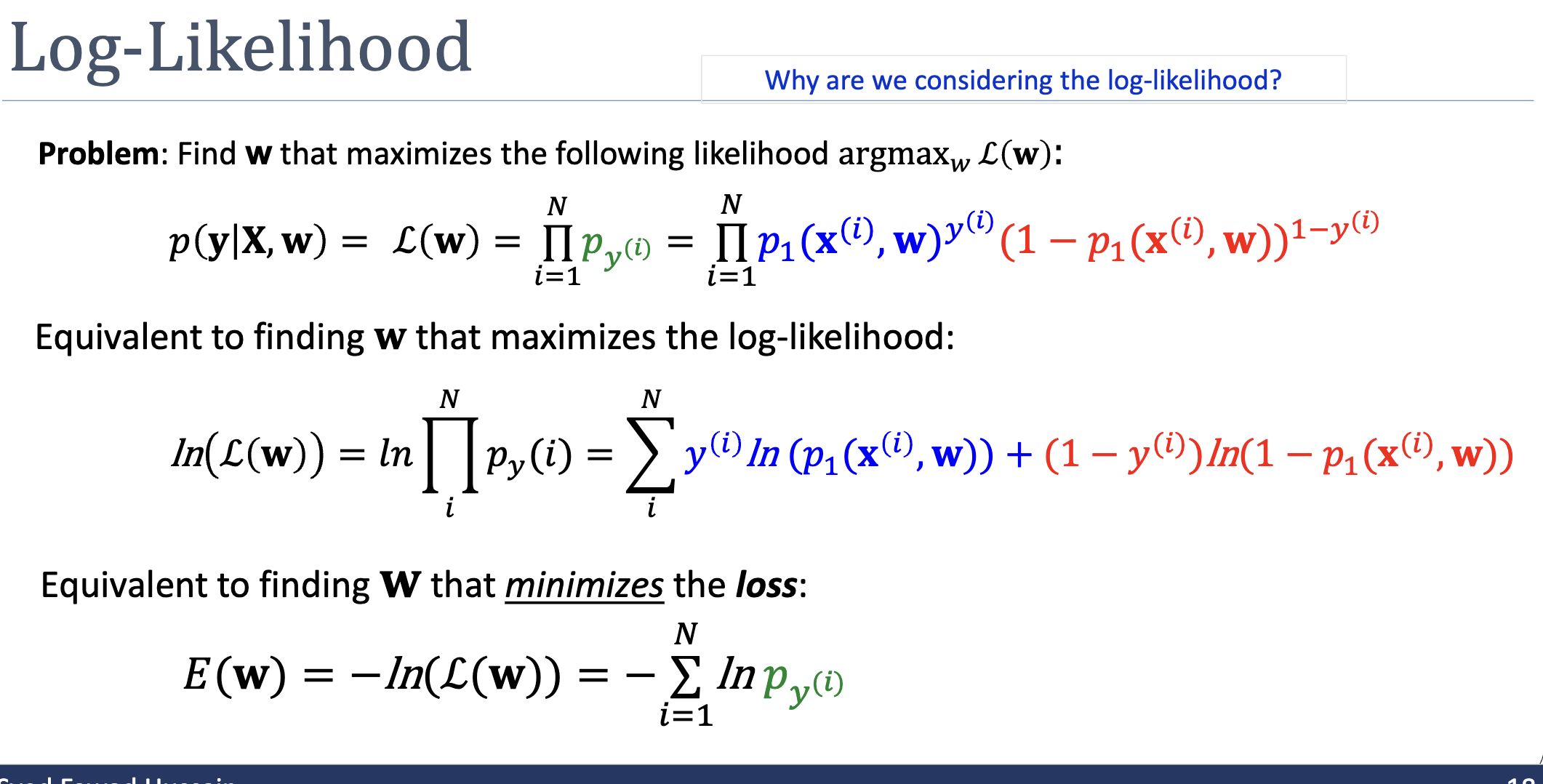
For binary classification with predicted probability $p_1=p(y=1\mid \mathbf{x},\mathbf{w})$ and ground-truth label $y\in \{0,1\}$, the cross-entropy loss over a training set of size $N$ is:

$E(\mathbf{w})=-{\sum }_{i=1}^N\left[y^{(i)}\ln p_1({\mathbf{x}}^{(i)},\mathbf{w})+(1-y^{(i)})\ln (1-p_1({\mathbf{x}}^{(i)},\mathbf{w}))\right]$

The two terms are a switch driven by the binary label:

• If $y^{(i)}=1$, only the first term survives: $-\ln p_1$.
• If $y^{(i)}=0$, only the second: $-\ln (1-p_1)$.

In both cases, you’re penalised by the negative log of the probability the model assigns to the correct class.

Behaviour

The shape of $-\ln p$ for $p\in (0,1]$ does most of the work:

Predicted probability of correct class	Loss contribution
$0.99$	$\approx 0.01$
$0.5$	$\approx 0.69$
$0.1$	$\approx 2.3$
$0.01$	$\approx 4.6$
$\to 0$	$\to \infty$

The loss explodes as the model confidently predicts the wrong class — confident wrongness is punished disproportionately, which is exactly what a calibrated probabilistic classifier should optimise.

Connection to Maximum Likelihood

Cross-entropy isn’t an arbitrary choice. It is exactly the negative log-likelihood under MLE. Starting from the likelihood and applying $-\ln$:

$\mathcal{L}(\mathbf{w})={\prod }_{i=1}^N{p}_1^{y^{(i)}}(1-p_1{)}^{1-y^{(i)}}$

$E(\mathbf{w})=-\ln \mathcal{L}(\mathbf{w})=-{\sum }_{i=1}^N\left[y^{(i)}\ln p_1+(1-y^{(i)})\ln (1-p_1)\right]$

Maximising likelihood ↔ minimising cross-entropy. Same optimum, different signs.

Why “Cross-Entropy”?

In information theory, the cross-entropy between two distributions $P$ (true) and $Q$ (predicted) over a discrete outcome $y$ is:

$H(P,Q)=-{\sum }_{y}P(y)\ln Q(y)$

For each training example, the true distribution is a one-hot — all probability mass on the actual label — and $Q$ is the model’s predicted distribution. The per-example cross-entropy reduces to $-\ln Q(y_{\text{true}})$, and the loss is the empirical sum across examples. So the loss measures the average dissimilarity between the model’s predicted distributions and the (one-hot) ground-truth distributions.

Convexity

The cross-entropy loss for logistic-regression is strictly convex in $\mathbf{w}$. This is the property that makes optimisation tractable: there is a single global minimum, and any reasonable iterative method (gradient descent, newton-raphson-method) will find it.

This convexity does not generalise to deeper models. A neural network with cross-entropy loss is non-convex in its parameters because the network’s output is a non-convex function of its weights — the loss itself is still convex in the output, but composing with the network breaks convexity.

Gradient

The gradient of the cross-entropy loss with respect to $\mathbf{w}$, when $p_1=\sigma ({\mathbf{w}}^{\top }\mathbf{x})$, is remarkably clean:

$\nabla E(\mathbf{w})={\sum }_{i=1}^N(p_1({\mathbf{x}}^{(i)},\mathbf{w})-y^{(i)}){\mathbf{x}}^{(i)}$

That is, the prediction error $(p_1-y)$ multiplied by the input vector, summed over the training set. The cleanness comes from a cancellation between the derivative of $-\ln p_1$ and the derivative of the sigmoid: the chain rule produces ${\sigma }^{\prime }(z)=\sigma (z)(1-\sigma (z))$, which exactly cancels the $1/p_1\cdot 1/(1-p_1)$ terms, leaving the residual.

Related

• maximum likelihood estimation — cross-entropy is the negative log-likelihood
• logistic-regression — cross-entropy’s primary user in this module
• gradient descent — the natural minimiser
• convex-function — the property that makes cross-entropy easy to optimise

Active Recall

For a single training example with $y=1$ and predicted $p_1=0.5$, what does the example contribute to the loss? What about $y=0$ with $p_1=0.5$?

Both contribute $-\ln (0.5)\approx 0.69$ — the maximum possible loss when the model is at chance level. This is the “natural” reference point: a model that always predicts $0.5$ gets a per-example loss of $\ln 2$.

Why does the loss go to infinity when the model predicts $p_1=0$ for an example with $y=1$?

When $y=1$, the loss term is $-\ln p_1$. As $p_1\to 0$, $-\ln p_1\to +\infty$. Information-theoretically: the model claimed “this outcome is impossible,” but it happened. Any finite penalty would be an under-statement of how badly that prediction misrepresented reality.

Show that the gradient of the per-example loss $-y\ln p_1-(1-y)\ln (1-p_1)$ with respect to $\mathbf{w}$ simplifies to $(p_1-y)\mathbf{x}$, given $p_1=\sigma ({\mathbf{w}}^{\top }\mathbf{x})$.

Let $z={\mathbf{w}}^{\top }\mathbf{x}$ so $p_1=\sigma (z)$. By the chain rule, $\partial p_1/\partial \mathbf{w}={\sigma }^{\prime }(z)\mathbf{x}=p_1(1-p_1)\mathbf{x}$. The derivative of $-y\ln p_1-(1-y)\ln (1-p_1)$ with respect to $p_1$ is $-y/p_1+(1-y)/(1-p_1)=(p_1-y)/(p_1(1-p_1))$. Multiplying by $\partial p_1/\partial \mathbf{w}$, the $p_1(1-p_1)$ factors cancel, leaving $(p_1-y)\mathbf{x}$.