maximum-likelihood-estimation-ml

A principle for fitting parametric models: choose the parameters that make the observed data most probable. For supervised learning, this turns “find the best $\mathbf{w}$” into a precise optimisation problem.

The Principle

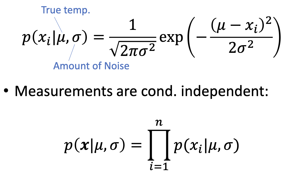
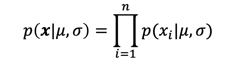
Given a parametric model $p(y\mid \mathbf{x},\mathbf{w})$ and a training set $\mathcal{T}=\{({\mathbf{x}}^{(i)},y^{(i)}){\}}_{i=1}^N$ drawn i.i.d. from the true distribution, the likelihood of the parameters is the joint probability of the observed labels:

$\mathcal{L}(\mathbf{w})=p(\mathbf{y}\mid \mathbf{X},\mathbf{w})={\prod }_{i=1}^{N}p(y^{(i)}\mid {\mathbf{x}}^{(i)},\mathbf{w})$

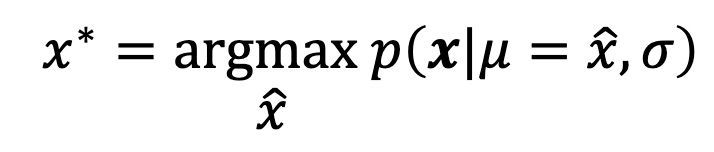
The maximum likelihood estimate is the parameter vector that maximises this:

${\mathbf{w}}^{\ast }=\arg {\max }_{\mathbf{w}}\mathcal{L}(\mathbf{w})$

Intuitively: of all the candidate $\mathbf{w}$‘s, pick the one for which the data we actually saw is the most plausible.

Probability vs Likelihood

The quantity $p(y\mid \mathbf{x},\mathbf{w})$ has two readings depending on what is fixed:

Reading	Fixed	Variable	Question answered
Probability	$\mathbf{w}$	$y$	”Given these parameters, how likely is this label?”
Likelihood	$y$	$\mathbf{w}$	”Given this observed label, how plausible are these parameters?”

In MLE, the data is observed and fixed; we vary $\mathbf{w}$ to find the best fit. The mathematical formula is identical; only the interpretation flips.

Why Take the Log?

Working directly with the product $\prod p_{y^{(i)}}$ is awkward for two reasons:

1. Numerical underflow. Multiplying $N$ probabilities (each $\le 1$) gives an absurdly small number that floating-point arithmetic represents as zero.
2. Calculus on products is messy. Differentiating a product of $N$ terms via the product rule blows up; differentiating a sum of $N$ terms is term-by-term.

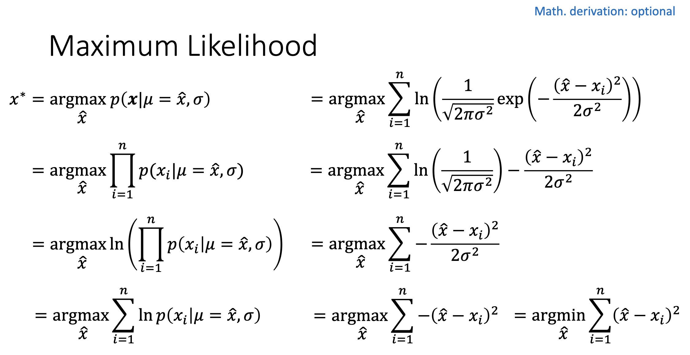
The fix is the monotonic logarithm. Since $\ln$ is strictly increasing, $\arg {\max }_{\mathbf{w}}\mathcal{L}(\mathbf{w})=\arg {\max }_{\mathbf{w}}\ln \mathcal{L}(\mathbf{w})$. The log-likelihood turns the product into a sum:

$\ln \mathcal{L}(\mathbf{w})={\sum }_{i=1}^N\ln p(y^{(i)}\mid {\mathbf{x}}^{(i)},\mathbf{w})$

Convention also prefers minimisation, so we negate to get the negative log-likelihood, which serves as a loss function:

$E(\mathbf{w})=-\ln \mathcal{L}(\mathbf{w})=-{\sum }_{i=1}^N\ln p(y^{(i)}\mid {\mathbf{x}}^{(i)},\mathbf{w})$

MLE for Logistic Regression

For logistic-regression, $p(y=1\mid \mathbf{x},\mathbf{w})=\sigma ({\mathbf{w}}^{\top }\mathbf{x})=p_1$ and $p(y=0\mid \mathbf{x},\mathbf{w})=1-p_1$. A single likelihood term, written compactly using the binary label, is:

$p_{y^{(i)}}=p_1^{y^{(i)}}(1-p_1{)}^{1-y^{(i)}}$

(When $y^{(i)}=1$ this reduces to $p_1$; when $y^{(i)}=0$ it reduces to $1-p_1$.) Plugging into the log-likelihood and negating gives the cross-entropy-loss:

$E(\mathbf{w})=-{\sum }_{i=1}^N\left[y^{(i)}\ln p_1({\mathbf{x}}^{(i)},\mathbf{w})+(1-y^{(i)})\ln (1-p_1({\mathbf{x}}^{(i)},\mathbf{w}))\right]$

So maximum likelihood and cross-entropy minimisation are the same problem for logistic regression — they differ only by a sign and a logarithm. Whichever lens you use, the optimal ${\mathbf{w}}^{\ast }$ is the same.

MLE Is the Source of Standard Loss Functions

A subtle point worth flagging: the loss function we minimise is not arbitrary — it falls out of MLE once you commit to a likelihood model. Different probabilistic assumptions yield different “standard” losses:

Likelihood model	$-\ln p(y\mid \mathbf{x},\mathbf{w})$ becomes	Standard name
Bernoulli ($y\in \{0,1\}$)	$-y\ln p_1-(1-y)\ln (1-p_1)$	Binary cross-entropy-loss
Categorical ($y$ one of $K$ classes)	$-{\sum }_k{y}_k\ln p_k$	Multi-class cross-entropy
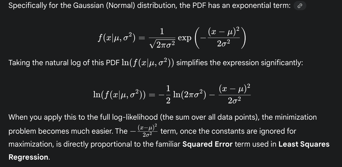
Gaussian noise ($y=f(\mathbf{x},\mathbf{w})+\epsilon$, $\epsilon \sim \mathcal{N}(0,{\sigma }^2)$)	$\frac{1}{2{\sigma }^2}(y-f(\mathbf{x},\mathbf{w}){)}^2+\text{const}$	Squared error / MSE
Laplace noise ($\epsilon \sim \text{Laplace}$)	$\tfrac{1}{b}	y - f(\mathbf{x}, \mathbf{w})
Poisson ($y\in \mathbb{N}$)	$f(\mathbf{x},\mathbf{w})-y\ln f(\mathbf{x},\mathbf{w})$	Poisson loss

The squared-error loss for linear regression isn’t a heuristic choice — it’s the negative log-likelihood under a Gaussian-noise model. The cross-entropy loss for logistic regression isn’t a heuristic — it’s the negative log-likelihood under a Bernoulli model. The principle is one (MLE); the loss is whatever the assumed likelihood produces.

This generality is why MLE shows up everywhere in modern ML. Picking a loss function is, implicitly, picking a noise model.

When Does MLE Work?

MLE has good theoretical properties — it’s consistent (recovers the true parameters in the infinite-data limit) and asymptotically efficient (achieves the lowest possible variance among unbiased estimators) under mild conditions.

It can fail when:

• The model is misspecified (the true distribution isn’t in the parametric family).
• Data is scarce relative to the number of parameters (MLE overfits).
• The likelihood has multiple maxima (in non-convex models like neural networks).

For logistic regression, the negative log-likelihood is strictly convex in $\mathbf{w}$, so MLE has a unique solution and any optimiser that converges to a critical point converges to it.

Related

• cross-entropy-loss — the negative log-likelihood for logistic regression
• logistic-regression — the model whose parameters MLE finds
• gradient descent — one way to actually solve the MLE optimisation
• supervised-learning — the broader framework MLE lives within

Active Recall

A model assigns probabilities $0.9,0.8,0.4,0.95,0.7$ to the correct labels of five training examples. Compute the likelihood and the negative log-likelihood. Which would you rather work with numerically, and why?

Likelihood: $0.9\times 0.8\times 0.4\times 0.95\times 0.7\approx 0.1915$. Negative log-likelihood: $-(\ln 0.9+\ln 0.8+\ln 0.4+\ln 0.95+\ln 0.7)\approx -(-0.105-0.223-0.916-0.051-0.357)\approx 1.652$. The log version is preferable: a sum of moderate numbers, rather than a product of values $\le 1$. With thousands of examples, the raw likelihood would underflow to zero; the log-likelihood remains a well-conditioned sum.

Why does maximising likelihood give the same answer as minimising negative log-likelihood?

Two reasons combine. First, $\ln$ is strictly monotonic, so $\arg {\max }_{\mathbf{w}}f(\mathbf{w})=\arg {\max }_{\mathbf{w}}\ln f(\mathbf{w})$. Second, negation flips max to min: $\arg {\max }_{\mathbf{w}}g(\mathbf{w})=\arg {\min }_{\mathbf{w}}-g(\mathbf{w})$. So $\arg \max \mathcal{L}=\arg \max \ln \mathcal{L}=\arg \min (-\ln \mathcal{L})$. The optimal ${\mathbf{w}}^{\ast }$ is invariant.

For binary logistic regression, write the likelihood term for a single training example $({\mathbf{x}}^{(i)},y^{(i)})$ in a way that handles both $y^{(i)}=0$ and $y^{(i)}=1$ in a single expression.

$p_{y^{(i)}}=p_1^{y^{(i)}}(1-p_1{)}^{1-y^{(i)}}$. When $y^{(i)}=1$: $p_1^1(1-p_1{)}^0=p_1$. When $y^{(i)}=0$: $p_1^0(1-p_1{)}^1=1-p_1$. The binary label acts as a switch via the exponents.