logistic-regression

A discriminative binary classifier that models the log-odds of class membership as a linear combination of features, producing calibrated probabilities via the sigmoid function.

Definition

Logistic regression models the probability of class 1 as:

$P(y=1\mid \mathbf{x},\mathbf{w})=\sigma ({\mathbf{w}}^{\top }\mathbf{x})=\frac{1}{1+e^{-{\mathbf{w}}^{\top }\mathbf{x}}}$

where $\mathbf{w}\in {\mathbb{R}}^{d+1}$ is the weight vector (including a bias term $w_0$ paired with a dummy input $x_0=1$) and $\sigma$ is the sigmoid function. Despite its name, logistic regression is a classification method, not a regression method.

Odds and the Logit

Before we can write down the model, we need a quantity that lives on the same scale as a linear combination — i.e., something that ranges over $(-\infty ,+\infty )$.

Odds are a natural intermediate step. The odds of class 1 are the ratio of its probability to the probability of class 0:

$o_1=\frac{p_1}{p_0}=\frac{p_1}{1-p_1}$

Concretely: if $p_1=0.7$ and $p_0=0.3$, then $o_1\approx 2.33$ — class 1 is about 2.3× more likely than class 0. If $p_1=p_0=0.5$, then $o_1=1$ — a coin flip. If $p_1=0.3$, then $o_1\approx 0.43$ — class 0 is more likely. The odds range over $[0,+\infty )$: still not the full real line.

Taking the logarithm of the odds gives the logit (log-odds), which maps $(0,1)\to (-\infty ,+\infty )$:

$\text{logit}(p_1)=\ln \frac{p_1}{1-p_1}$

Now we can safely set this equal to the linear combination:

$\text{logit}(p_1)=\ln \frac{p_1}{1-p_1}={\mathbf{w}}^{\top }\mathbf{x}$

Both sides are unbounded real numbers. Solving for $p_1$ yields the sigmoid:

$p_1=\frac{e^{{\mathbf{w}}^{\top }\mathbf{x}}}{1+e^{{\mathbf{w}}^{\top }\mathbf{x}}}=\frac{1}{1+e^{-{\mathbf{w}}^{\top }\mathbf{x}}}$

Why not model $\ln (p_1)={\mathbf{w}}^{\top }\mathbf{x}$ directly? Because $\ln (p_1)\le 0$ for any valid probability — logarithm is only unbounded in one direction, so it still can’t match ${\mathbf{w}}^{\top }\mathbf{x}$ on the positive side. The logit is the fix precisely because it is symmetric and fully unbounded.

Odds Ratio Interpretation

Since $\ln (o_1)={\mathbf{w}}^{\top }\mathbf{x}$, the odds of class 1 are $o_1=e^{{\mathbf{w}}^{\top }\mathbf{x}}$. A unit increase in feature $x_j$ (all else equal) changes the logit by $w_j$, which multiplies the odds by $e^{w_j}$. This is why the effect of features on odds is multiplicative, not additive.

This gives logistic regression a direct interpretability advantage: each weight $w_j$ tells you exactly how much feature $x_j$ shifts the class-1 odds. A large positive weight means the feature strongly favours class 1; a large negative weight strongly favours class 0.

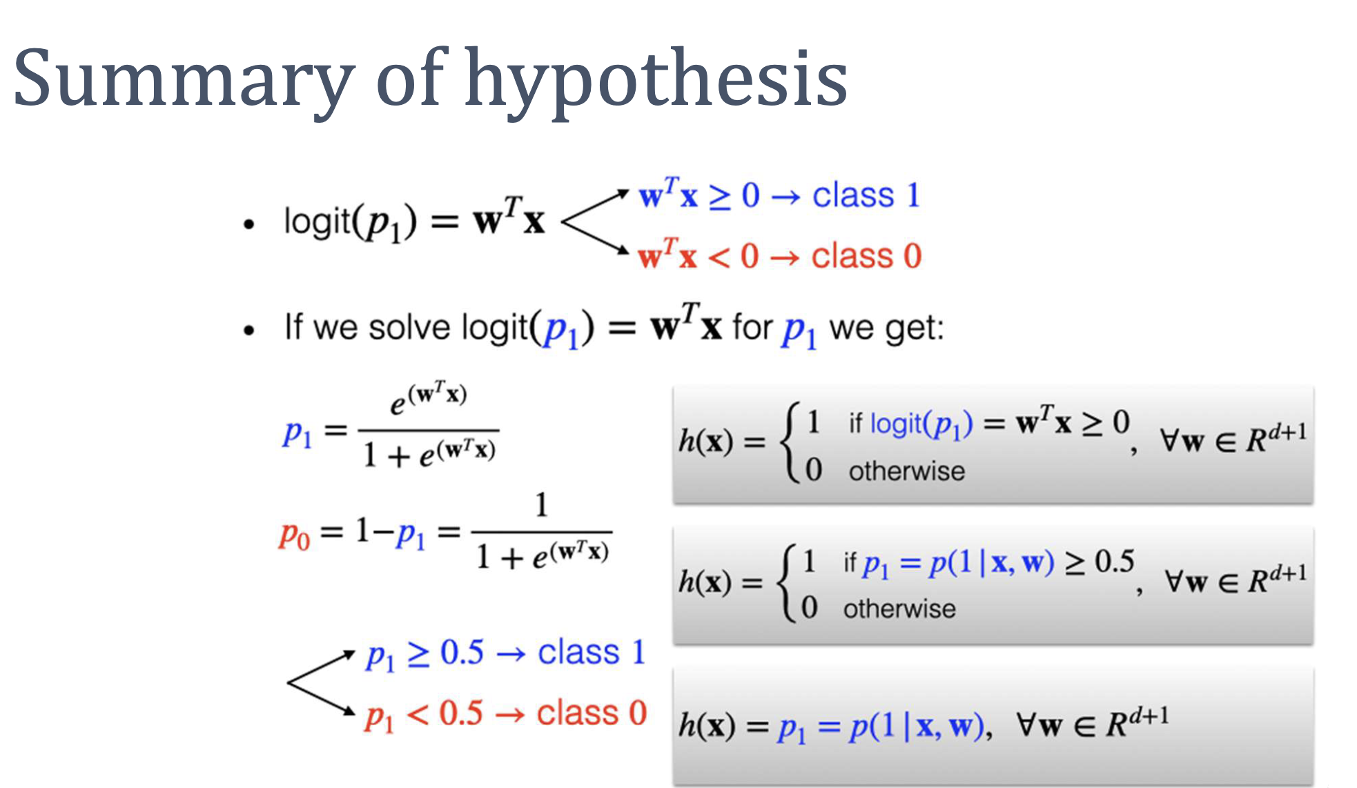
Hypothesis Set and Classification

The hypothesis set is $\mathcal{H}=\{h(\mathbf{x})=\sigma ({\mathbf{w}}^{\top }\mathbf{x})\mid \mathbf{w}\in {\mathbb{R}}^{d+1}\}$. Learning means finding the weight vector $\mathbf{w}$ that best fits the training data.

Classification follows from probability thresholding:

• ${\mathbf{w}}^{\top }\mathbf{x}\ge 0⟹p_1\ge 0.5⟹$ predict class 1
• ${\mathbf{w}}^{\top }\mathbf{x}<0⟹p_1<0.5⟹$ predict class 0

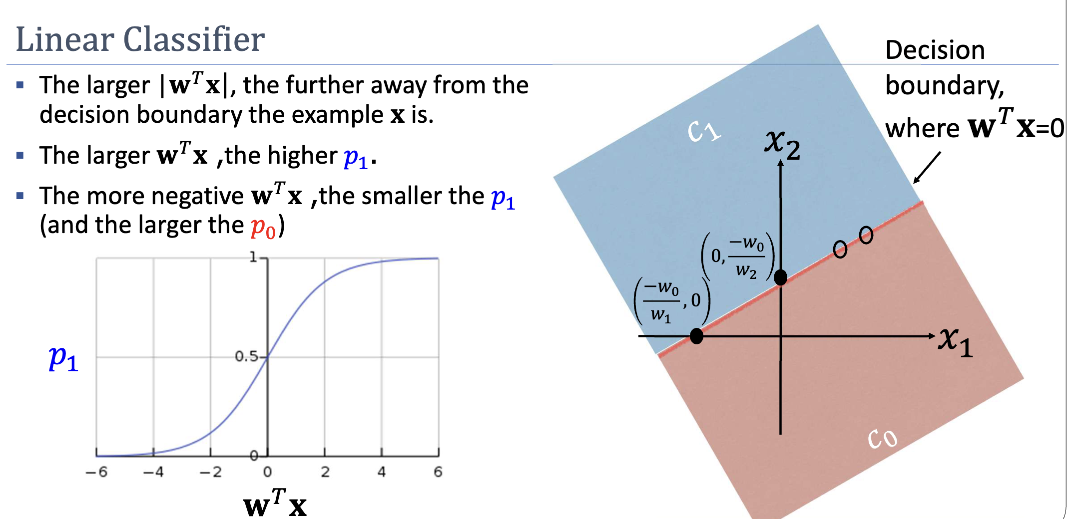
The decision boundary is the hyperplane ${\mathbf{w}}^{\top }\mathbf{x}=0$. Points far from this boundary (large $|{\mathbf{w}}^{\top }\mathbf{x}|$) have probabilities close to 0 or 1 — the model is confident. Points near the boundary (${\mathbf{w}}^{\top }\mathbf{x}\approx 0$) have $p_1\approx 0.5$ — the model is uncertain.

Discriminative Nature

Logistic regression is a discriminative classifier: it directly models $P(y\mid \mathbf{x})$ without modelling how the features themselves are generated. This contrasts with generative classifiers that model $P(\mathbf{x}\mid y)\cdot P(y)$ and apply Bayes’ rule.

Worked Example

Setup: Binary classification with 2 input features. Learned weights: ${\mathbf{w}}^{\top }=(0.1,0.2,0.6)$. New instance: ${\mathbf{x}}^{\top }=(1,1,3)$ (where $x_0=1$ is the dummy variable).

Step 1 — Linear combination:

${\mathbf{w}}^{\top }\mathbf{x}=(0.1)(1)+(0.2)(1)+(0.6)(3)=0.1+0.2+1.8=2.1$

Step 2 — Classification decision:

Since ${\mathbf{w}}^{\top }\mathbf{x}=2.1\ge 0$, predict class 1.

Step 3 — Probability:

$p_1=\frac{e^{2.1}}{1+e^{2.1}}=\frac{8.166}{9.166}\approx 0.891$

The model assigns roughly 89% probability to class 1.

Strengths and Limitations

Strengths:

• Calibrated probabilities, not just labels. $p_1$ is a real probability, useful when downstream decisions depend on confidence — medical risk, fraud scoring, threshold tuning.
• Fast inference. Classification reduces to one dot product and a threshold check; trivially deployable on embedded systems.
• Compact model. Storing $\mathbf{w}$ is $d+1$ floats. No training data needs to be retained at inference (unlike kNN or SVM, which need support vectors).
• Interpretable coefficients. Each $w_j$ has a direct odds-ratio meaning ($e^{w_j}$); the magnitude indicates feature importance if features are on the same scale and not collinear.
• Extends to multi-class. Softmax regression generalises directly; the optimisation stays convex.

Limitations:

• Linear decision boundary. Without a basis expansion, logistic regression cannot capture curved or disjoint class regions. For non-linearly separable data, a hyperplane in the original space will leave some points misclassified by construction.
• Logistic-form assumption. The model assumes $P(y\mid \mathbf{x})$ has the specific shape $\sigma ({\mathbf{w}}^{\top }\mathbf{x})$. Real conditional distributions may not — in which case the predicted probabilities are miscalibrated even when the classification accuracy is reasonable.
• Sensitivity to multicollinearity. When features are highly correlated, the estimated weights become unstable: many different $\mathbf{w}$ vectors give nearly the same predictions, and small changes in the training data swing the weights wildly. Predictions can stay accurate, but coefficient interpretation becomes unreliable.
• Perfect separability is awkward. When the training data is linearly separable, the maximum-likelihood weights are unbounded (they grow to infinity to make $\sigma$ saturate). Regularisation (L2 or L1) is the standard fix.

Related

• sigmoid function — the activation that converts logit to probability
• decision boundary — the geometric separator produced by logistic regression
• supervised-learning — the framework logistic regression operates within
• discriminative-vs-generative-models — where logistic regression sits in the taxonomy
• non-linear-transformation — the standard fix for the linear-boundary limitation

Active Recall

Why can't we simply set $P(y=1\mid \mathbf{x})={\mathbf{w}}^{\top }\mathbf{x}$ and call it a day?

The linear combination ${\mathbf{w}}^{\top }\mathbf{x}$ is unbounded — it can take any value in $(-\infty ,+\infty )$. Probabilities must lie in $[0,1]$. Setting the two equal would produce “probabilities” like $-500$ or $47$. The logit function bridges this gap: we model the log-odds (which is also unbounded) as ${\mathbf{w}}^{\top }\mathbf{x}$, then invert via the sigmoid to recover a valid probability.

Given ${\mathbf{w}}^{\top }=(-0.5,1.0,-2.0)$ and ${\mathbf{x}}^{\top }=(1,3,1)$, compute ${\mathbf{w}}^{\top }\mathbf{x}$, state the predicted class, and calculate $p_1$.

${\mathbf{w}}^{\top }\mathbf{x}=(-0.5)(1)+(1.0)(3)+(-2.0)(1)=-0.5+3.0-2.0=0.5$. Since $0.5\ge 0$, predict class 1. $p_1=1/(1+e^{-0.5})=1/(1+0.6065)\approx 0.622$.

In a logistic regression model, feature $x_3$ has weight $w_3=0.5$. If $x_3$ increases by 1 unit (all else equal), how do the odds of class 1 change? Why is the change multiplicative, not additive?

The odds are multiplied by $e^{0.5}\approx 1.649$ — roughly a 65% increase. The relationship is multiplicative because the logit is a log-odds: $\ln (o_1)={\mathbf{w}}^{\top }\mathbf{x}$. Adding $w_3$ to the logit is equivalent to multiplying the odds by $e^{w_3}$, since $\exp (\ln (o_1)+w_3)=o_1\cdot e^{w_3}$.

Logistic regression finds a decision boundary, but it doesn't guarantee that the boundary is "good" in any geometric sense. What weakness does this expose, and what later algorithm addresses it?

Logistic regression finds a hyperplane that separates the classes (if the data is linearly separable), but it doesn’t maximize the margin — the distance from the nearest training points to the boundary. A small margin means the classifier is fragile to small perturbations. Support Vector Machines (SVMs) explicitly maximize the margin, producing a more robust boundary.