Allowing Mistakes: Soft Margins and How to Actually Solve the QP

THE CRUX: Week 4 gave us a kernelised SVM dual that is mathematically clean — but it assumes the data is linearly separable in $\varphi$-space, and even when it is, the $N$-variable QP is too expensive to solve directly. Two open ends. How do we (a) handle data that can't be separated cleanly, and (b) actually compute the optimum at scale?

The fix is a pair of complementary changes. (a) Introduce a slack variable ${\xi }^{(n)}\ge 0$ for each training example, relaxing the constraint $y^{(n)}h({\mathbf{x}}^{(n)})\ge 1$ to $y^{(n)}h({\mathbf{x}}^{(n)})\ge 1-{\xi }^{(n)}$, and add $C{\sum }_n{\xi }^{(n)}$ to the objective. The hyperparameter $C$ trades margin width against violation tolerance. The dual is identical to last week’s except for one detail: $a^{(n)}$ is now bounded above by $C$ — the box constraint. (b) Solve the QP via Sequential Minimal Optimization (SMO): pick a pair of multipliers $(a^{(i)},a^{(j)})$, solve the two-variable subproblem analytically, clip to feasibility, repeat. Two variables is the minimum required because the equality constraint ${\sum }_n{a}^{(n)}{y}^{(n)}=0$ pins any single multiplier in place.

---

Last week ended with the kernelised dual:

$\arg {\max }_{\mathbf{a}}{\sum }_n{a}^{(n)}-\frac{1}{2}{\sum }_{n,m}{a}^{(n)}{a}^{(m)}{y}^{(n)}{y}^{(m)}k({\mathbf{x}}^{(n)},{\mathbf{x}}^{(m)})\text{s.t. }{a}^{(n)}\ge 0,{\sum }_n{a}^{(n)}{y}^{(n)}=0$

Two unanswered questions hang over it:

1. What if no separating hyperplane exists? With a Gaussian kernel, $\varphi$-space is infinite-dimensional, so some separator almost always exists — but it may be over-specific to the training data. With a linear kernel and overlapping classes, no separator exists at all. Either way: hard-margin SVM is brittle.
2. How do we actually solve this? $N$ variables, with a Gram matrix that’s $N\times N$, dense, and stored in memory. Off-the-shelf QP runs out of room past a few thousand examples.

Week 5 closes both. Part 1 (Monday) introduces slack and the soft-margin dual. Part 2 (Tuesday) introduces SMO.

Part 1: Soft-Margin SVM

From Hard to Soft

The hard-margin constraint says “every point is at least one margin-unit on the correct side”:

$y^{(n)}h({\mathbf{x}}^{(n)})\ge 1\forall n$

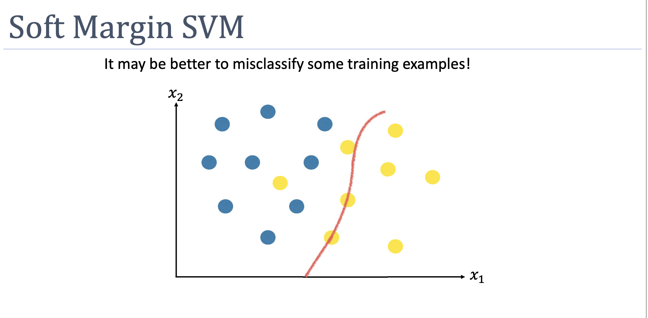
If even one point violates this, the constraint set is empty. The relaxation: each point gets a personal violation budget ${\xi }^{(n)}\ge 0$:

$y^{(n)}h({\mathbf{x}}^{(n)})\ge 1-{\xi }^{(n)}$

Now the constraint is always satisfiable — set ${\xi }^{(n)}$ large enough and any classification works. To stop the optimiser from making slack infinite, penalise it in the objective:

$\boxed{\arg \underset{\mathbf{w},b,\mathbf{\xi }}{\min }\frac{1}{2}\Vert \mathbf{w}{\Vert }^2+C\sum _{n=1}^N{\xi }^{(n)}\text{s.t. }{y}^{(n)}h({\mathbf{x}}^{(n)})\ge 1-{\xi }^{(n)},{\xi }^{(n)}\ge 0}$

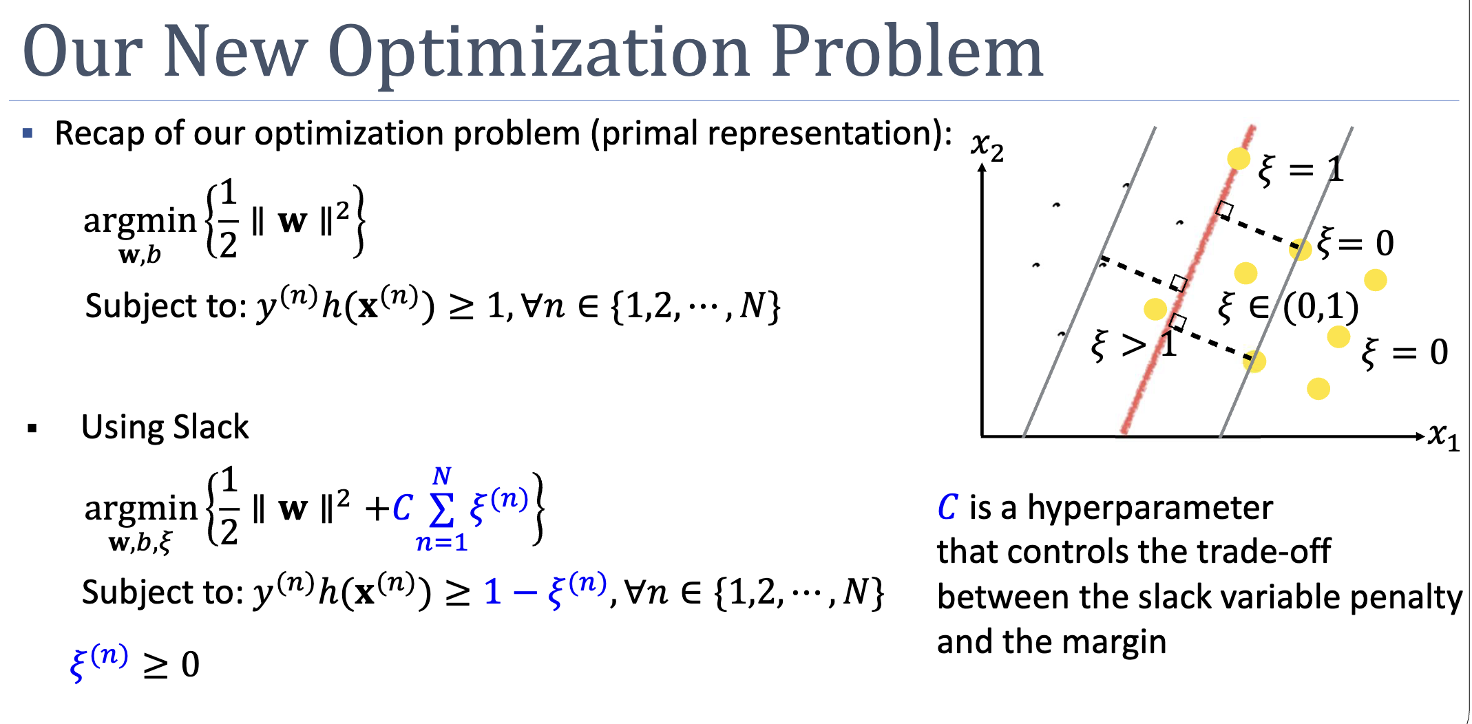
The hyperparameter $C>0$ sets the slack price. Large $C$ → expensive slack → narrow margin, behaves like hard-margin. Small $C$ → cheap slack → wide margin, many margin-violators tolerated.

Reading ${\xi }^{(n)}$ Geometrically

The value of ${\xi }^{(n)}$ at the optimum encodes where point $n$ sits:

${\xi }^{(n)}$	Position
$=0$	Outside or on the margin envelope (constraint slack)
$\in (0,1)$	Inside the margin envelope, correctly classified
$=1$	Exactly on the decision boundary
$>1$	Misclassified — wrong side of the boundary

A clean identity: ${\xi }^{(n)}=\max (0,1-y^{(n)}h({\mathbf{x}}^{(n)}))$. This is exactly the hinge loss — soft-margin SVM is L2-regularised hinge-loss minimisation.

Slack is a value, not a count

The objective penalises ${\sum }_n{\xi }^{(n)}$ — the total magnitude of violation, not the number of violators. One badly-misclassified point ($\xi =1.5$) costs more than three margin-grazers ($\xi =0.4$ each). The formulation cares about depth, not breadth.

The Margin Definition Changes

In hard-margin SVM, the margin was $1/\Vert \mathbf{w}\Vert$ defined as the distance from the boundary to the closest training point (canonically rescaled to $yh=1$). With soft margin, “closest training point” is no longer well-defined — some points lie inside the margin. The margin is now simply $1/\Vert \mathbf{w}\Vert$ as a definitional choice, decoupled from any particular training point.

The Dual: Almost Unchanged

Apply Lagrangian relaxation as before. We now have two sets of multipliers — $a^{(n)}\ge 0$ for the margin constraint and ${\beta }^{(n)}\ge 0$ for ${\xi }^{(n)}\ge 0$:

$L=\frac{1}{2}\Vert \mathbf{w}{\Vert }^2+C{\sum }_n{\xi }^{(n)}+{\sum }_n{a}^{(n)}(1-{\xi }^{(n)}-y^{(n)}h({\mathbf{x}}^{(n)}))-{\sum }_n{\beta }^{(n)}{\xi }^{(n)}$

Setting partials of $L$ to zero gives:

• ${\mathbf{w}}^{\ast }={\sum }_n{a}^{(n)}{y}^{(n)}\varphi ({\mathbf{x}}^{(n)})$ (same as hard-margin)
• ${\sum }_n{a}^{(n)}{y}^{(n)}=0$ (same)
• New: $C-a^{(n)}-{\beta }^{(n)}=0$, i.e., ${\beta }^{(n)}=C-a^{(n)}$

The third relation, combined with ${\beta }^{(n)}\ge 0$ and $a^{(n)}\ge 0$, gives the box constraint:

$\boxed{0\le a^{(n)}\le C}$

Substituting back, ${\xi }^{(n)}$ and ${\beta }^{(n)}$ vanish entirely. The dual is identical to the hard-margin one, with one upper-bound difference:

$\arg {\max }_{\mathbf{a}}{\sum }_n{a}^{(n)}-\frac{1}{2}{\sum }_{n,m}{a}^{(n)}{a}^{(m)}{y}^{(n)}{y}^{(m)}k({\mathbf{x}}^{(n)},{\mathbf{x}}^{(m)})\text{s.t. }0\le a^{(n)}\le C,{\sum }_n{a}^{(n)}{y}^{(n)}=0$

The kernel trick still applies. Predictions still use $h(\mathbf{x})={\sum }_{n\in S}{a}^{(n)}{y}^{(n)}k(\mathbf{x},{\mathbf{x}}^{(n)})+b$. The entire effect of slack collapses, in dual form, to the single change $a^{(n)}\le C$.

Three Categories of Support Vector

KKT complementary slackness gives two equations:

$a^{(n)}(1-{\xi }^{(n)}-y^{(n)}h({\mathbf{x}}^{(n)}))=0$ $(C-a^{(n)}){\xi }^{(n)}=0$

These split training points into three regimes:

$a^{(n)}$	${\xi }^{(n)}$	Type	Position
$0$	$0$	Not a support vector	Strictly outside the margin
$(0,C)$	$0$	Margin support vector	Exactly on the margin: $yh=1$
$C$	$\ge 0$	Bound support vector	Anywhere from on-margin to misclassified

When $0<a^{(n)}<C$, then ${\beta }^{(n)}=C-a^{(n)}>0$, which forces ${\xi }^{(n)}=0$ via the second condition; combined with $a^{(n)}>0$ this pins the point exactly on the margin via the first. When $a^{(n)}=C$, the second condition is automatically satisfied for any ${\xi }^{(n)}\ge 0$, so the point can sit anywhere — including misclassified.

This is why only margin support vectors are used to compute $b$:

$b=\frac{1}{|M|}{\sum }_{n\in M}\left(y^{(n)}-{\sum }_{m\in S}{a}^{(m)}{y}^{(m)}k({\mathbf{x}}^{(n)},{\mathbf{x}}^{(m)})\right),M=\{n:0<a^{(n)}<C\}$

Bound SVs ($a=C$) have $yh=1-{\xi }^{(n)}\ne 1$ in general, so substituting them gives the wrong $b$.

Sparsity, Weakened But Preserved

In hard-margin SVM, only on-margin points have $a^{(n)}>0$ — typically a tiny fraction. In soft-margin SVM, every margin violator also has $a^{(n)}=C$, expanding the support set. But examples comfortably outside the margin still have $a^{(n)}=0$ and contribute nothing to predictions. Sparsity is weaker but not lost.

Part 2: Sequential Minimal Optimization

The dual is a convex QP with $N$ variables, an $N\times N$ Gram matrix, box constraints, and a linear equality. Off-the-shelf QP solvers run in $O(N^3)$ time and store the full Gram matrix in memory. For $N=10^5$ that’s already 80GB and trillions of operations. We need a method that exploits the structure.

The Decomposition Idea

Instead of solving for all $N$ multipliers at once, fix most of them and optimise over a small subset. With two at a time, the subproblem has a closed-form analytic solution.

Why two and not one? The equality constraint ${\sum }_n{a}^{(n)}{y}^{(n)}=0$ couples the multipliers. Picking just $a^{(m)}$ to update with everything else fixed forces:

$a^{(m)}{y}^{(m)}=-{\sum }_{n\ne m}{a}^{(n)}{y}^{(n)}=\text{constant}$

so $a^{(m)}$ is pinned. Two multipliers can move while preserving the constraint — a change in $a^{(i)}$ is absorbed by a compensating change in $a^{(j)}$.

The SMO Loop

Initialise a^(n) = 0 for all n.       # feasible: 0 ∈ [0,C], Σ a y = 0
Repeat until convergence:
    Pick (i, j) heuristically.
    Compute a^(j,new) analytically.
    Clip a^(j,new) to [L, H] for box feasibility.
    Recover a^(i,new) from the equality constraint.

Convergence is signalled when no example violates KKT within tolerance.

The Analytic Update

Substituting $a^{(i)}$ as a function of $a^{(j)}$ (via $a^{(i)}{y}^{(i)}+a^{(j)}{y}^{(j)}=\zeta$) into the dual objective and differentiating w.r.t. $a^{(j)}$:

$\boxed{a^{(j,\text{new})}=a^{(j)}+\frac{y^{(j)}(E^{(i)}-E^{(j)})}{k({\mathbf{x}}^{(i)},{\mathbf{x}}^{(i)})+k({\mathbf{x}}^{(j)},{\mathbf{x}}^{(j)})-2k({\mathbf{x}}^{(i)},{\mathbf{x}}^{(j)})}}$

where $E^{(n)}=f({\mathbf{x}}^{(n)})-y^{(n)}$ is the prediction error on example $n$.

The denominator $k_{ii}+k_{jj}-2k_{ij}=\Vert \varphi ({\mathbf{x}}^{(i)})-\varphi ({\mathbf{x}}^{(j)}){\Vert }^2$ is the squared distance between the two examples in feature space. The numerator scales with the error disagreement. Far-apart examples with very different errors produce big steps.

Clipping

The candidate $a^{(j,\text{new})}$ may exceed $[0,C]$, or push $a^{(i)}$ (computed from it) outside the box. The feasible interval $[L,H]$ for $a^{(j)}$ depends on whether $y^{(i)}=y^{(j)}$:

• Same labels ($y^{(i)}=y^{(j)}$, line $a^{(i)}+a^{(j)}=\zeta /y$): $L=\max (0,a^{(j)}+a^{(i)}-C),H=\min (C,a^{(j)}+a^{(i)})$
• Different labels ($y^{(i)}\ne y^{(j)}$): $L=\max (0,a^{(j)}-a^{(i)}),H=\min (C,a^{(j)}-a^{(i)}+C)$

Then clip:

$a^{(j,\text{new\&clipped})}=\mathrm{clip}(a^{(j,\text{new})},L,H)$

and recover $a^{(i,\text{new})}=(\zeta -a^{(j,\text{new\&clipped})}{y}^{(j)})/y^{(i)}$.

Picking the Pair: Heuristics

Convergence is guaranteed for any selection — but speed is hugely heuristic-dependent. Standard recipe:

For $a^{(i)}$ (the first): Alternate between (1) random selection among examples violating KKT within tolerance $e$, and (2) random selection among margin SVs ($0<a<C$) violating KKT. Strategy 2 keeps the search on the active set; strategy 1 occasionally checks bound multipliers.

For $a^{(j)}$ (the second): Try in order until a positive improvement in $\tilde{L}$ is observed:

1. Maximum step heuristic. Pick the $j$ that maximises $|E^{(i)}-E^{(j)}|$ — approximates the largest update size.
2. Iterate over non-bound multipliers.
3. Iterate over the entire training set.
4. If still no improvement, replace $a^{(i)}$ and try again.

Errors $E^{(n)}$ are cached and updated incrementally.

KKT Conditions, Restated

In SMO terms, the optimum is characterised entirely by $a^{(n)}$:

Condition	Geometric meaning
$a^{(n)}=0⟺y^{(n)}h({\mathbf{x}}^{(n)})\ge 1$	Outside margin; not a SV
$0<a^{(n)}<C⟺y^{(n)}h({\mathbf{x}}^{(n)})=1$	On margin; margin SV
$a^{(n)}=C⟺y^{(n)}h({\mathbf{x}}^{(n)})\le 1$	On, inside, or violating margin; bound SV

When every example satisfies its KKT condition within tolerance, the dual is at its optimum.

What Could Go Wrong

• $C$ too large. Acts as hard-margin in disguise. Inherits all the overfitting and brittleness problems we introduced soft margin to avoid.
• $C$ too small. Slack is essentially free. The decision boundary collapses — any classification satisfies the constraints with cheap-enough $\xi$. The model underfits, possibly degenerating to “always predict the majority class.”
• No margin support vectors. If every SV is at $a=C$, the formula for $b$ has no inputs. Pick any of them and accept the resulting $b$.
• Numerical issues in SMO when ${\mathbf{x}}^{(i)}\approx {\mathbf{x}}^{(j)}$. The denominator $k_{ii}+k_{jj}-2k_{ij}\to 0$. Skip the pair.
• Lazy SMO heuristics. Random-random pair selection still converges, but may be 10×–100× slower than max-step. The heuristics matter.

---

Concepts Introduced This Week

• soft-margin-svm — SVM with slack-relaxed constraints; introduces hyperparameter $C$; dual differs from hard-margin only in the box constraint $a^{(n)}\le C$.
• slack-variables — per-example violation budgets ${\xi }^{(n)}\ge 0$; equal hinge loss at the optimum; enable SVM on non-separable data.
• sequential-minimal-optimization — decomposition algorithm for the SVM dual; iteratively updates pairs of multipliers analytically; two is the minimum because of the equality constraint.

Connections

• Builds on week-04 — uses the same Lagrangian / KKT / kernel machinery; the dual has the same form except for the box constraint.
• Builds on support-vector-machine and kernel-trick — soft margin is a relaxation, not a replacement; combined with kernels (especially Gaussian) it is the default sklearn.svm.SVC.
• Builds on kkt-conditions — complementary slackness now gives a three-way support-vector classification (non-SV / margin-SV / bound-SV) instead of two-way.
• Sets up later weeks: regularisation framework ($C$ is one example of the bias-variance trade-off knob); generalisation theory (margin-based bounds explain why widening the margin via small $C$ can improve test error); model selection (cross-validating $C$, $\sigma$, kernel choice).

Open Questions

• How do we choose $C$ (and the kernel hyperparameters) in practice? Cross-validation, but on what scale and grid?
• Why does SMO converge — what guarantees the analytic two-variable updates strictly increase $\tilde{L}$ until KKT is satisfied? (Convexity of $\tilde{L}$ + careful pair selection; the formal proof is in Platt’s original paper.)
• For multi-class problems, how does soft-margin SVM extend? (One-vs-rest, one-vs-one, Crammer–Singer — covered in later weeks or as background reading.)