weight-initialization

Where the weights start matters. Set them all to the same value and the network never learns; set them to values too large or too small and the gradients explode or vanish from the first step. Modern initialisation schemes draw small random values whose spread is matched to the activation function used downstream.

Why constant initialisation fails

Suppose every weight in a hidden layer is set to the same value (zero, one, anything). For a fixed input, every neuron in that layer computes the same pre-activation, the same activation, and — by symmetry of the gradient — the same update. After one step they’re all still equal. They remain interchangeable forever, learning the same feature in parallel. The hidden layer has the expressive power of a single neuron, regardless of how wide it is.

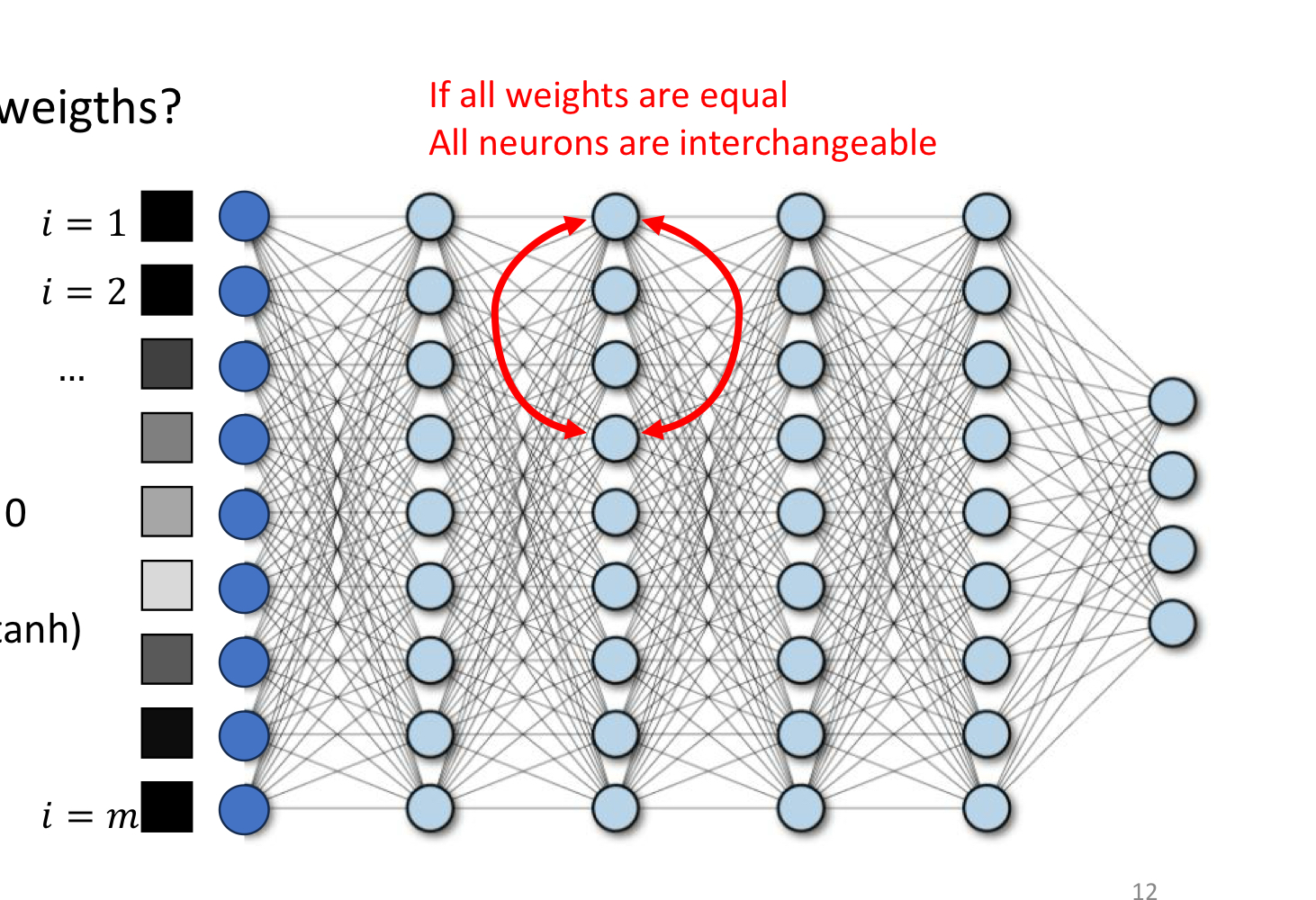
The picture is exactly this: identical weights mean every red neuron is functionally the same neuron. We want different parts of the network to specialise — to play different roles — and that requires breaking the symmetry from the very first step.

Random initialisation

The fix is to draw weights from a probability distribution so that no two neurons start equal:

• Uniform on $[-a,a]$ for some small $a$.
• Normal with mean $0$ and a chosen standard deviation $\sigma$. This is the more common default.

Biases are typically initialised to zero. The bias doesn’t contribute to symmetry between neurons within a layer (it’s a per-neuron offset), so a constant choice is fine.

The remaining question: what scale of random values? Too small and the activations shrink layer by layer until the signal is lost. Too large and the activations blow up. The “right” scale depends on the activation function and the layer width.

Scale-aware initialisation

Two schemes are standard, named after their inventors. Both pick a variance for the weights such that activations and gradients keep roughly constant variance from layer to layer.

Xavier (Glorot) initialisation. Designed for $\tanh$ and sigmoid:

$\text{Var}(w)=\frac{2}{n_{\text{in}}+n_{\text{out}}}$

where $n_{\text{in}}$ and $n_{\text{out}}$ are the input and output sizes of the layer.

He (Kaiming) initialisation. Designed for ReLU. Because ReLU zeros out half its inputs on average, the variance has to be doubled to compensate:

$\text{Var}(w)=\frac{2}{n_{\text{in}}}$

These look like minor numerical tweaks but they make a real difference. With matched initialisation, very deep networks (tens of layers) can be trained; with mismatched initialisation they often fail to make progress.

TIP — Match the init to the activation

The rough rule: He for ReLU, Xavier for tanh/sigmoid. Modern frameworks (PyTorch, TensorFlow) implement both as one-line calls (torch.nn.init.kaiming_normal_, xavier_uniform_, etc.). The default initialisation in PyTorch’s nn.Linear is already Kaiming uniform, calibrated for ReLU.

Why scale matters: gradient flow at depth

The same chain-rule argument that motivates non-saturating activations applies to initialisation. The forward pass multiplies activations by weight matrices layer after layer; the backward pass multiplies gradients by the same matrices. If the typical weight magnitude is too large, both grow exponentially with depth (exploding gradients). If it’s too small, both shrink to zero (vanishing gradients). Xavier and He pick the variance that keeps both flows roughly stationary across layers — neither shrinking nor growing.

This pairs with batch normalisation and skip connections, which give further safeguards against gradient instability deeper into training. Initialisation gets the network safely past step zero; the other tricks keep it on track.

Related

• activation-functions — the choice that determines which initialisation scheme to use
• normalization — addresses the same scale problem at run time, layer by layer
• residual-connection — another structural fix for vanishing/exploding gradients in deep networks
• backpropagation — the mechanism through which bad initialisation poisons learning

Active Recall

Why can't you initialise all the weights of a hidden layer to zero (or any constant)?

All neurons would compute the same pre-activation, hence the same activation, hence the same gradient, hence the same weight update. They would remain identical for every training step — the layer would have the expressive power of a single neuron no matter how wide it is. Random initialisation breaks this symmetry so neurons can specialise.

For a layer with ReLU activation, why does He initialisation use $\text{Var}(w)=2/n_{\text{in}}$ instead of the $1/n_{\text{in}}$ that would balance variance for a linear layer?

ReLU zeros out negative pre-activations — on average, half of them. That halves the variance of the layer’s outputs compared to a linear layer with the same weights. To keep activation variance constant from layer to layer, you have to double the weight variance to compensate. That’s the factor of 2 in He initialisation.

A 30-layer network is initialised with $\sigma =1$ (large). Predict what happens during the first forward pass and the first backward pass.

Forward pass: each layer multiplies its input by a weight matrix with large entries, so activations grow geometrically with depth. By layer 30 they’re astronomically large, often saturating activations or producing NaNs. Backward pass: gradients multiply by the same large matrices in reverse, exploding similarly. Either the loss is undefined or the first parameter update is huge and useless. The fix is to scale $\sigma$ down by the inverse-square-root of layer width (Xavier/He).

The biases of a network can be initialised to zero without breaking symmetry, even though zeroing the weights does. Why is that?

The symmetry-breaking requirement is between different neurons in the same layer — they must compute different things from the same input. The bias is a per-neuron offset, not a coupling between neurons; setting all biases to zero doesn’t make two neurons compute the same function unless their weights are also identical. Since the weights are random, the symmetry is already broken — the biases just start neutral.