normalization

Networks compute summations of products. If the inputs to one layer are on the scale of hundreds and the next layer’s weights aren’t tiny, the next layer’s pre-activations will be enormous — and once an activation function saturates or a gradient explodes, learning stalls. Normalisation keeps numbers in a sane range, both at the input and inside the network.

Why raw inputs are dangerous

Take an 8-bit greyscale image: every pixel is an integer in $[0,255]$. Feed it directly into a layer whose weights are $\sim \mathcal{N}(0,1)$. The pre-activation $z={\sum }_i{w}_i{x}_i$ is a sum of hundreds of such products and easily reaches several thousand in magnitude. Apply an activation:

• ReLU: the output is in the thousands. The next layer multiplies again and the values keep growing.
• Sigmoid/tanh: $z$ is so far from zero that the function saturates — derivative effectively zero, no gradient.

Either way the network either explodes or stops learning. The fix is preprocessing the input so values cluster around zero with a small spread.

Three input normalisation schemes

Three common ways to rescale a real-valued input feature $x$:

Scheme	Formula	Output range
Fixed scaling	$x^{\prime }=x/255$ (for 8-bit images)	$[0,1]$
Min-max	$x^{\prime }=(x-x_{\min })/(x_{\max }-x_{\min })$	$[0,1]$
Z-score	$x^{\prime }=(x-\mu )/\sigma$	mean 0, std 1

Z-score normalisation is the most common in deep learning. The mean $\mu$ and standard deviation $\sigma$ are computed from the training set and reused at test time. The result lands inputs near the “useful” zero region of common activation functions (ReLU’s elbow, sigmoid’s steep central section).

TIP — Compute statistics on training data only

$\mu$ and $\sigma$ are properties of the training distribution. Recomputing them from validation or test data would leak information from those splits into the model’s preprocessing — a subtle form of train/test contamination. Always compute statistics once on training data and apply the same shift and scale at validation and test time.

Why input normalisation isn’t enough

Normalising the input fixes layer 1. But layer 2 receives layer 1’s outputs — and as layer 1 trains, its weights change, so its output distribution drifts. Layer 2 is now chasing a moving target: by the time it has adapted to one input distribution, layer 1 has shifted to a new one. This is internal covariate shift, and it gets worse with depth: layer 10 in a 20-layer network has nine layers of drift to track.

The cure is to normalise inside the network, after every layer’s pre-activations. That’s batch normalisation.

Batch normalisation

Place a normalisation operation between a layer’s linear part ($z=Wx+b$) and its activation function. For each mini-batch of $m$ examples, compute the mean and variance of $z$ across the batch:

${\mu }_B=\frac{1}{m}{\sum }_{i=1}^m{z}_i,{\sigma }_B^2=\frac{1}{m}{\sum }_{i=1}^m(z_i-{\mu }_B{)}^2$

Normalise each example using these batch statistics:

${\hat{z}}_i=\frac{z_i-{\mu }_B}{\sqrt{{\sigma }_B^2+ϵ}}$

The $ϵ$ ($\sim 10^{-5}$) prevents division by zero when the batch happens to have constant pre-activations. After this step, $\hat{z}$ has mean 0 and variance 1 across the batch.

The learnable scale and shift

Forcing every layer’s outputs to be exactly mean 0 and variance 1 is too restrictive — sometimes the network really does want differently-scaled activations. So batch norm adds two learnable parameters per channel, $\gamma$ and $\beta$:

$y_i=\gamma {\hat{z}}_i+\beta$

$\gamma$ and $\beta$ let the model re-scale and re-centre the normalised activations — even undoing normalisation entirely if helpful (set $\gamma ={\sigma }_B$, $\beta ={\mu }_B$). The point isn’t to hand-tune the scale; it’s to let the network, not the human, decide whether to keep the normalisation, undo it, or end up somewhere in between.

TIP — Why $\gamma$ and $\beta$ are learnable

Without them, batch norm forces a hard zero-mean unit-variance constraint at every layer — that constraint can hurt the network if the optimal pre-activation distribution is genuinely different. Adding $\gamma$ and $\beta$ as learnable parameters means the network, not the human, decides whether to keep the normalisation, undo it, or end up somewhere in between. Crucially, even when the network learns to undo the normalisation, gradient descent now starts from a well-scaled state instead of an arbitrary one.

Train time vs test time

At training time, ${\mu }_B$ and ${\sigma }_B$ come from the current mini-batch. At test time you may only have one example — there’s no batch to compute statistics from. The standard fix:

1. During training, maintain a running average of ${\mu }_B$ and ${\sigma }_B^2$ across mini-batches.
2. At test time, freeze and use these running estimates instead of computing fresh batch statistics.

So batch norm has two modes of operation: training mode (computes per-batch stats, updates running averages) and evaluation mode (uses frozen running averages). Forgetting to switch modes is one of the most common batch-norm bugs.

Batch norm for CNNs: per-channel statistics

A convolution layer’s output is a 4D tensor of shape $(\text{batch},\text{channels},H,W)$. Because the same filter slid over every spatial position to produce that channel, every spatial location of one channel is computed by the same weights — so the natural statistic to normalise is the entire channel pooled across batch and space. For each channel, compute $\mu$ and $\sigma$ over the batch dimension and the spatial dimensions, then learn one $\gamma ,\beta$ pair per channel.

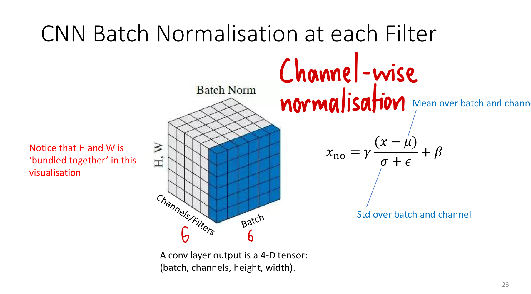
The diagram shows the 4D tensor flattened to 3D for visualisation: each cube has axes for batch, channel, and spatial (H and W collapsed into one axis). The shaded slab in batch normalisation is “all batches × all spatial positions” of one channel — that’s the slice over which mean and variance are computed. The result is channel-wise normalisation: each filter’s outputs get their own statistics, but those statistics aggregate information from every example and every pixel that channel produced.

Why batch norm helps

Empirically: faster convergence, less sensitivity to initialisation, mild regularisation effect (each example sees noisy statistics from its mini-batch peers, similar in spirit to dropout). The mechanism is gradient flow — well-scaled pre-activations keep activation derivatives in the useful regime, especially for ReLU.

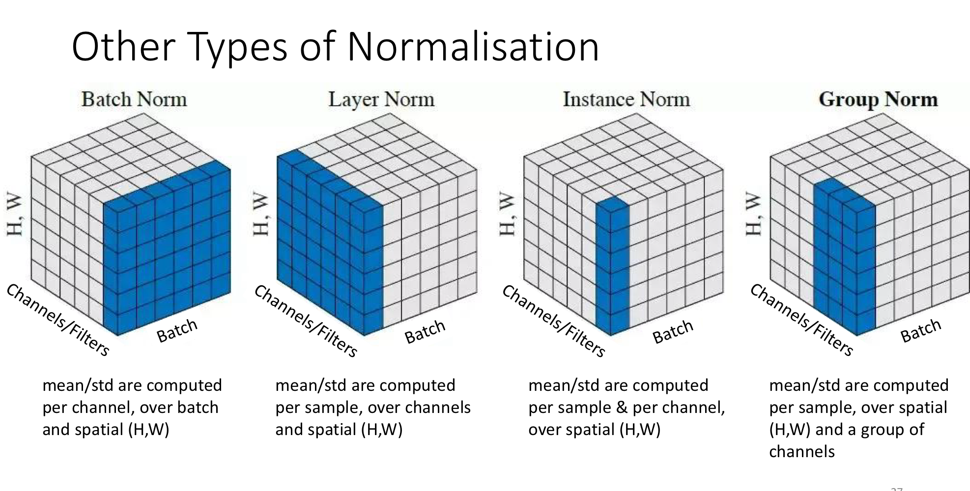
Other types of normalisation

The “slab” picture generalises. Different choices of which dimensions to pool over give different normalisation schemes, useful when batch normalisation’s batch-level statistics are unreliable (small batches) or unwanted (style transfer).

Scheme	Statistics computed over	When it shines
Batch norm	Batch + spatial (H, W); per channel	Standard CNN training with reasonable batch sizes
Layer norm	Channels + spatial; per sample	Recurrent networks, transformers — independent of batch size
Instance norm	Spatial only; per sample, per channel	Style transfer (each image’s style is normalised independently)
Group norm	Spatial + a manually chosen channel group; per sample	Small-batch CNN training, where batch norm’s statistics get noisy

All four use the same $\hat{z}=(z-\mu )/\sqrt{{\sigma }^2+ϵ}$ formula plus learnable $\gamma ,\beta$. Only the shape of the slab over which $\mu$ and $\sigma$ are computed changes. Batch norm is the default for CNNs at typical batch sizes; the others exist for specific cases where batch norm’s reliance on batch statistics is a problem.

Related

• activation-functions — normalisation keeps inputs in the useful (non-saturating) regime of these
• weight-initialization — addresses the same scale problem at $t=0$; normalisation maintains it through training
• gradient-descent-variants — mini-batch SGD is the context where “batch” in batch norm makes sense
• backpropagation — gradients flow through normalisation as just another differentiable operation
• dropout — another technique with regularisation as a side effect; the two are commonly combined

Active Recall

A network's first hidden layer receives raw pixel values in $[0,255]$ and uses a sigmoid activation. Predict what happens to the activations and gradients in the first forward and backward pass.

Pre-activations $z=\sum w_i{x}_i$ are very large in magnitude (hundreds × small weights still gives big sums). The sigmoid saturates: outputs are pinned at $\approx 1$ (or $\approx 0$ for negative pre-activations), and the derivative ${\sigma }^{\prime }(z)=\sigma (z)(1-\sigma (z))$ is essentially zero. The gradient signal through this layer is destroyed before training even begins. Z-score normalisation of the input prevents this by bringing values into the steep central region of the sigmoid where gradients are non-trivial.

What is internal covariate shift, and why is it a particular problem for deep networks?

As earlier layers update, their output distributions change — but those distributions are the inputs to later layers, so each later layer is constantly adapting to a moving target. The deeper the network, the more layers of accumulated drift. Layer 1’s small change cascades through layers 2, 3, … 10. Batch normalisation fixes this by re-centring each layer’s pre-activations to mean 0 / variance 1 every step, so downstream layers always see a stable input distribution.

Why does batch normalisation include the learnable scale $\gamma$ and shift $\beta$? Wouldn't simple zero-mean unit-variance normalisation be enough?

Forcing every layer to have exactly that distribution is a hard constraint, and sometimes the network’s optimal representation is not at mean 0, variance 1. The learnable $\gamma ,\beta$ let the network choose its scale and shift — including the choice to undo the normalisation entirely if that’s what minimises the loss. The benefit isn’t that the final activations end up normalised; it’s that gradient descent always starts from a well-scaled state and can move away from it deliberately.

During training, batch norm uses the current mini-batch's mean and variance. What does it use at test time, and why can't you just use the test sample's statistics?

At test time it uses running averages of ${\mu }_B$ and ${\sigma }_B^2$ accumulated across all training mini-batches. You can’t use the test sample’s statistics because (a) at inference you may have a single example, with no batch to compute statistics from, and (b) test-time predictions should depend only on the input, not on what other examples happen to be batched alongside it. Frozen training-time statistics give deterministic, batch-independent inference.

For a convolution layer, batch norm computes statistics across the batch dimension and the spatial dimensions, but separately for each channel. Why per-channel and not per-pixel?

Because the same filter produced every spatial position of a given channel — a $3\times 3$ kernel at position $(5,5)$ uses the same weights as that kernel at $(50,50)$. Those outputs share statistics; normalising them together respects the convolution’s weight-sharing structure. Normalising per-pixel would be too granular (no batch effect within a pixel) and would break the symmetry that made convolution efficient in the first place.

When would you use group normalisation instead of batch normalisation?

When the batch size is small. Batch norm’s statistics become noisy with few examples — at batch size 1, ${\sigma }_B=0$ exactly and the operation degenerates. Group norm computes statistics over a manually chosen group of channels within a single sample, so it doesn’t depend on batch size at all. This matters for memory-constrained training (large image segmentation, video models) where batches of 32+ aren’t feasible.