residual-connection

A simple structural change — add the input $x$ back to the output of a small block of layers, so the block computes $F(x)+x$ instead of $F(x)$. The mathematical effect is to reframe the layer’s job: instead of transforming $x$ into something new, it learns the residual correction to $x$. The optimisation effect is that gradients now have a direct path backwards. Together these enable training networks 50, 100, even 1000 layers deep — something that simply stacking plain layers cannot achieve.

The problem: deeper networks are harder, not easier

Naive intuition says: a deeper network is at least as expressive as a shallow one (the deeper net can simulate the shallow net by learning identity transformations in its extra layers, then doing whatever the shallow net does). So a 56-layer network should match or beat a 20-layer network on training error.

It doesn’t.

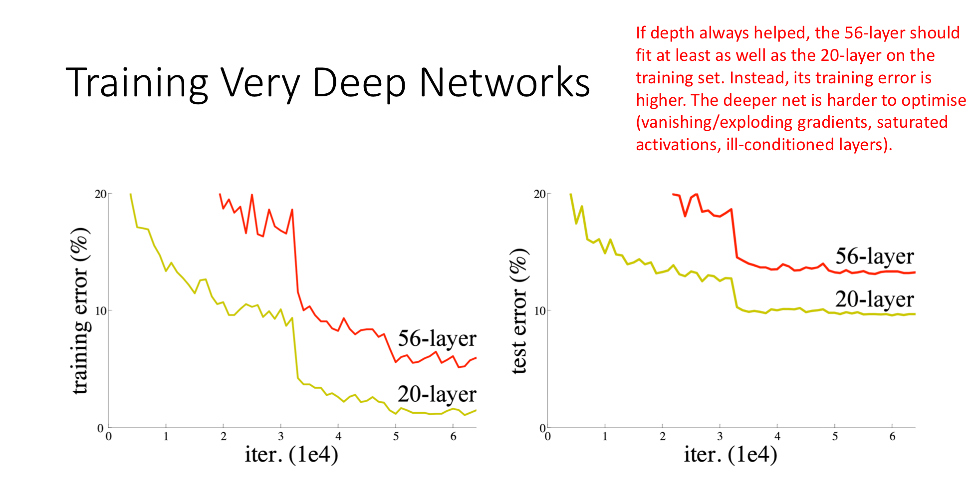
The 56-layer plain network has higher training error than the 20-layer plain network — the deeper net is failing to learn what it should be capable of. This is the degradation problem. It is not overfitting (the gap shows up on training data, not just test data). The deeper network is harder to optimise:

• Vanishing/exploding gradients through long chains of multiplications.
• Saturated activations in the middle of the network.
• Ill-conditioning — the loss landscape becomes a treacherous tangle of cliffs and ravines.

The extra 36 layers, in principle capable of doing nothing useful, cannot even learn to do nothing with naive optimisation.

TIP — The broken telephone

The intuition for why gradients fail in deep networks is the children’s game of “telephone”: the error signal has to travel backwards from the output through every layer to reach the input, and at each hop it gets multiplied, distorted, attenuated. By the time it reaches layer 1 of a 56-layer network, the signal is unrecognisable noise. Early layers never get the memo on how to update. The skip connection is, in this analogy, handing the person at the end of the line a written copy of the original message — bypassing the chain of distortions entirely.

The fix: residual blocks

He et al. (2016) introduced ResNet (Residual Network) with a deceptively simple structural change:

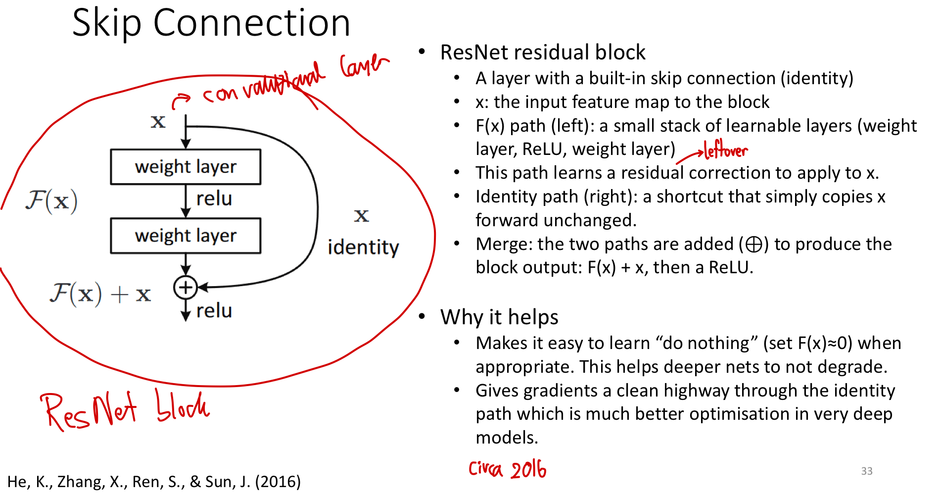
Take a small stack of layers — typically a few weight layers and a ReLU. Call its function $F(x)$. Add a shortcut connection that bypasses the stack entirely, copying the input $x$ unchanged. Merge the two paths by addition:

$y=F(x)+x$

Inside the block, $F(x)$ — the residual function — represents the change the block applies to $x$, not the full output. The original information $x$ flows through untouched along the identity path; the layers just learn what correction to apply.

That’s the entire idea. Stack many such blocks and you have a ResNet.

ASIDE — Why "residual"

Residual = “what’s left over”. If the ideal output of the block is some target $H(x)$, a plain block has to learn the entire $H$ from scratch. A residual block only has to learn $H(x)-x=F(x)$ — the correction that turns $x$ into $H(x)$. When the ideal correction is small (and it often is, especially deep into the network), learning a small $F$ is much easier than learning a complex $H$ directly.

Why this fixes degradation

Two distinct mechanisms make residual blocks easier to train.

Reason 1: identity is the easy default

A plain block has to learn very precise weights to implement the identity mapping ($y=x$) — the weights have to compose to exactly the identity matrix, threading through ReLU non-linearities. That’s a hard target.

A residual block implements identity by setting $F(x)=0$, which is trivially achievable by zeroing the inner weights:

$y=0+x=x$

So in a deep ResNet, layers that genuinely have nothing to add can effectively turn themselves off, leaving the network as if those layers weren’t there. This guarantees a deeper ResNet is at least as good as a shallower one — adding more residual blocks can only help, never hurt. This is the “do no harm” principle.

Reason 2: gradient highway

Backpropagation through $y=F(x)+x$ propagates gradients through both paths and adds them. The identity path is just multiplication by 1, so gradients flow through it with no scaling, no saturation, no vanishing:

$\frac{\partial L}{\partial x}=\frac{\partial L}{\partial y}\cdot \left(1+\frac{\partial F}{\partial x}\right)$

The “+1” is the identity-path contribution. Even if $\partial F/\partial x$ is tiny (vanishing through the inner layers), the +1 keeps the gradient alive. Stack 100 residual blocks and the gradient at layer 1 still has a clean unmodulated path back from the loss — a “gradient superhighway”.

This is structurally analogous to what ReLU’s $f^{\prime }(z)=1$ does for non-saturating activations, but operating on whole blocks instead of single neurons.

The visual evidence

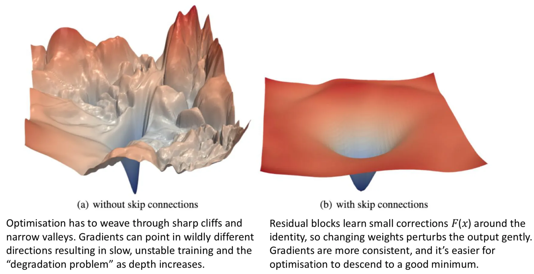
The loss landscape — the geography that the optimiser has to navigate — is dramatically smoother with skip connections. The left plot is the loss surface of a deep plain network: jagged cliffs, sharp peaks, narrow valleys where gradient descent gets stuck. The right plot is the same network with skip connections added: a smooth bowl with a clear path to the minimum. Same task, same depth, very different optimisation difficulty.

Comparing ResNet to plain deep networks

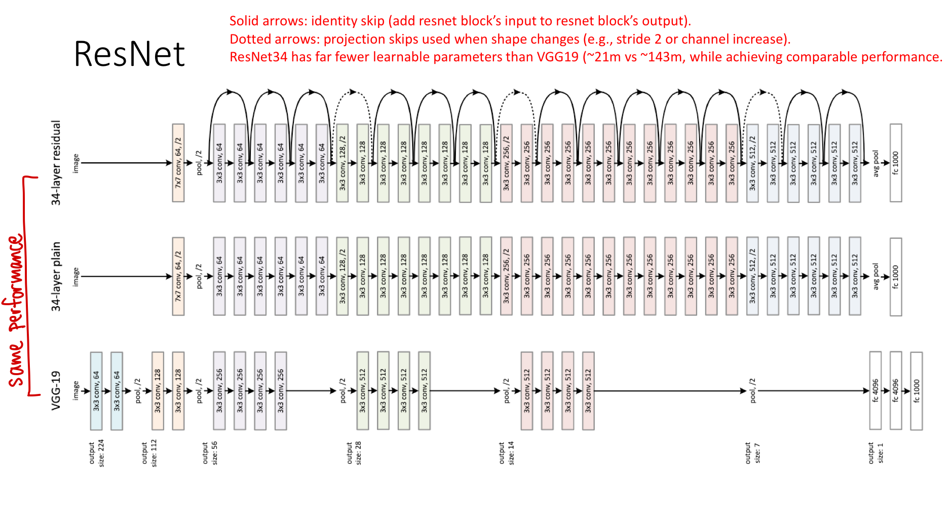
The original ResNet paper compared a 34-layer ResNet against VGG19 (19 layers, plain) and a 34-layer plain network. Two findings:

1. The 34-layer plain network was worse than VGG19 — degradation in action. More layers, worse performance.
2. The 34-layer ResNet matched or beat VGG19 despite using only ~21M parameters versus VGG19’s ~143M. Skip connections let depth pay off, and the deeper network was also more parameter-efficient.

Solid arrows are identity skip connections (same shape on both sides, just add). Dotted arrows are projection shortcuts — used when the residual block changes the spatial size or channel count, so the identity needs a small linear projection to match. The projection adds a few learnable parameters but preserves the residual structure.

Where residual connections show up

ResNet was the first big example, but the pattern is now everywhere:

• ResNet (image classification): the original use, identity shortcuts within conv blocks.
• U-Net (segmentation): skip connections from encoder to decoder, but using concatenation instead of addition. The role is similar — preserve high-resolution information that would otherwise be lost.
• Transformers: every attention block and every FFN block in a transformer is wrapped in a residual connection. Without them, transformers would be untrainable at modern depths (12, 24, 96 layers).
• U-Net variants combining both (sometimes called “Res-U-Net”): residual connections inside encoder/decoder blocks and concatenation-based skips between them.

The pattern — preserve the input alongside the transformed version, let the network learn what to add or change — has become a fundamental architectural primitive.

Related

• convolutional-neural-network — ResNet is the canonical CNN that put residual connections to work
• backpropagation — the chain-rule argument for why the +1 in the identity gradient saves vanishing gradients
• activation-functions — ReLU’s non-saturating gradient is a per-neuron analogue of what residual connections do per-block
• normalization — batch norm typically sits inside each residual block in modern ResNets
• u-net — a network architecture using a different flavour of skip connection (concatenation) for segmentation

Active Recall

The "degradation problem" is not overfitting, even though both involve a deeper model performing worse. Explain the difference.

Overfitting is when the deeper model fits training data better than the shallow one but fails on test data — the gap is between train and test. Degradation is when the deeper model fits training data itself worse than the shallow one — it’s failing to learn at all, not failing to generalise. The 56-layer plain net underperforms the 20-layer plain net on the training set, which means it lacks the optimisation efficiency to even reach the same fit, let alone overfit. The fix is structural (residual connections), not regularisation.

Write the formula for a residual block. Explain what $F(x)$ represents and why this is called "residual".

$y=F(x)+x$. Here $x$ is the input to the block, $F(x)$ is the output of a small stack of inner layers (e.g. weight–ReLU–weight), and $y$ is the block’s output. $F(x)$ represents the residual — the small correction the block applies to $x$ on its way to becoming $y$. Rather than learning the full transformation $H(x)=y$, the block learns just the difference $F(x)=H(x)-x$. When the ideal correction is small (or zero), this is much easier to learn than the full $H$.

Why does adding skip connections make it easy for a deep network to learn the identity mapping in unneeded layers, and why does that matter?

A plain block computes $y=F(x)$; making this the identity requires the inner layers to compose exactly to the identity matrix through ReLUs — a hard, precise target. A residual block computes $y=F(x)+x$; making this the identity requires only $F(x)=0$, which is achieved by zeroing the inner weights — easy. This matters because it means adding more residual blocks to a network never hurts: blocks that aren’t needed can effectively turn themselves off. Plain networks lack this guarantee, which is why naive depth degrades performance.

Use the chain rule to show how the identity path in a residual block keeps gradients from vanishing, even when the inner layers' gradient $\partial F/\partial x$ is tiny.

For $y=F(x)+x$, the gradient of the loss w.r.t. $x$ is $\frac{\partial L}{\partial x}=\frac{\partial L}{\partial y}\cdot \left(1+\frac{\partial F}{\partial x}\right)$. The “+1” comes from the identity path’s derivative. Even if $\partial F/\partial x$ vanishes through saturated activations or shrunken weights, the +1 contribution survives and the gradient at $x$ is at least $\partial L/\partial y$. Stack many residual blocks and gradients still flow clean through the identity additions, instead of being multiplicatively killed layer by layer.

ResNet-34 (residual, ~21M parameters) outperforms VGG19 (plain, ~143M parameters) on ImageNet. What does this tell us about the value of depth versus width?

Depth, properly used, is a more efficient way to spend parameters than width. ResNet-34 has more layers but each layer is narrower than VGG19’s, and skip connections make the depth tractable. The result: stronger representational hierarchy with fewer total weights. The lesson informed all subsequent architectures — modern image models prefer many narrow layers (with residual or other depth-enabling tricks) over a few wide ones.