activation-functions

The non-linearity between layers is what gives a network expressive power beyond a single linear map. The choice of activation affects how gradients flow during training — and the wrong choice can stop a deep network from learning at all.

Why a non-linearity at all

At each neuron, the raw weighted sum $z=w_0+w_1{x}_1+\cdots +w_D{x}_D$ is a linear function of the inputs. The activation $a=f(z)$ is what decides — non-linearly — how strongly that neuron fires.

Stack two linear layers: $a^2=W^2(W^{1}x+b^1)+b^2=(W^2{W}^1)x+(W^2{b}^1+b^2)$. Composing linear maps gives a linear map. No matter how many layers you stack, without non-linearity between them, the network is mathematically equivalent to a single linear layer — same expressive power as a single perceptron.

The activation function $f(\cdot )$ in $a^{\ell }=f(W^{\ell }{a}^{\ell -1}+b^{\ell })$ is what breaks this collapse. Each activation introduces a non-linearity that subsequent linear layers can’t undo. Stacked layers can now represent functions far richer than any single linear layer.

What non-linearity buys you geometrically

The algebraic statement “composing linear maps gives a linear map” has a sharp geometric consequence. A purely linear network can only carve input space with hyperplanes — straight lines in 2D, flat planes in 3D, flat $(D-1)$-surfaces in general. That’s the entire hypothesis class, regardless of depth.

Insert a non-linearity between layers and the boundary is no longer constrained to be flat. It can:

• curve to follow the contour of a class,
• bend sharply where two classes meet at an angle,
• loop to enclose a cluster from all sides,
• wrap around interleaved data like spirals or concentric rings.

Each layer applies a small distortion to the representation; stacking layers compounds these distortions. A two-layer net can already form curved boundaries; a deeper net can carve nested or looping regions that no shallow linear classifier could ever express. This is the geometric face of universal approximation — and it is bought entirely by $f(\cdot )$.

The four canonical activations

Sigmoid

$\sigma (z)=\frac{1}{1+e^{-z}}$

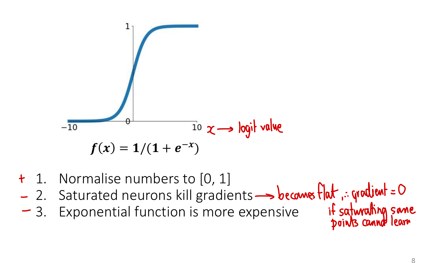
See sigmoid function for the full treatment. Range $(0,1)$, useful when outputs need to be probabilities. Differentiable, with derivative ${\sigma }^{\prime }(z)=\sigma (z)(1-\sigma (z))$, max value $0.25$ at $z=0$.

Problems for hidden layers:

• Saturation kills gradients. For $|z|\gg 0$, ${\sigma }^{\prime }(z)\approx 0$. Hidden units in saturation stop learning.
• Not zero-centred. Outputs are always positive, which means gradients of weights all have the same sign per training step — slows convergence.
• Expensive. The exponential takes more compute than simple max operations.

Modern networks use sigmoid almost exclusively at output layers (for binary classification probabilities), not in hidden layers.

Tanh

$\tanh (z)=\frac{e^z-e^{-z}}{e^z+e^{-z}}$

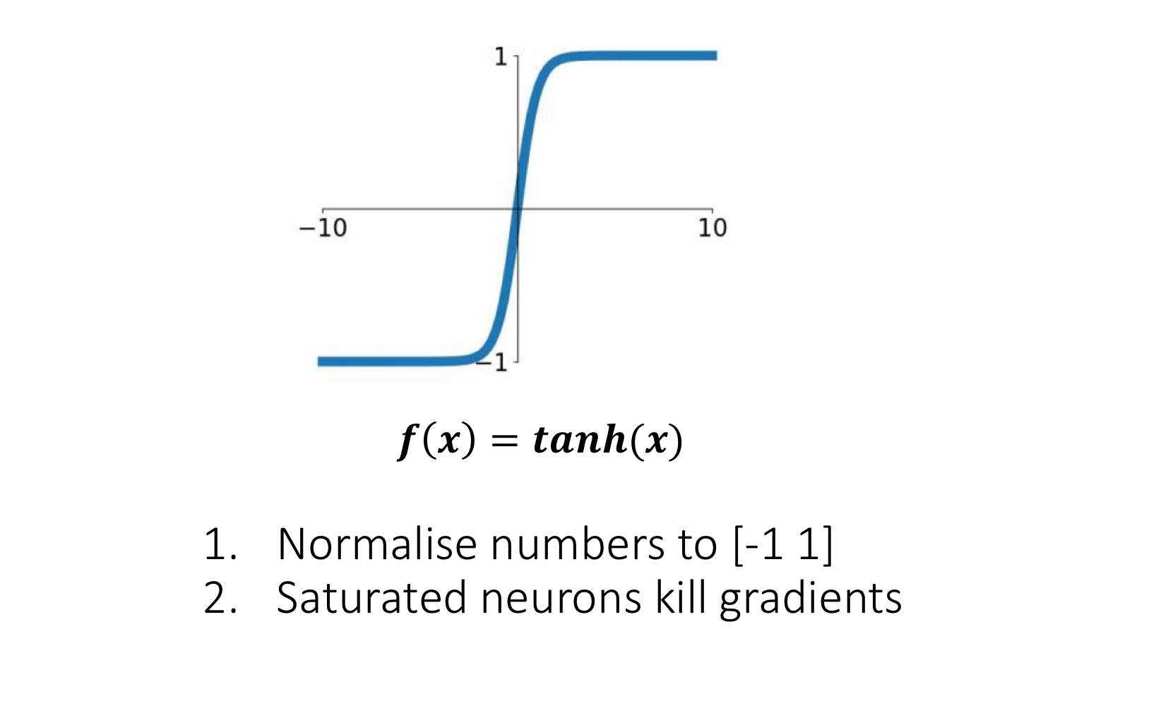
Squashed to $(-1,1)$ instead of $(0,1)$. Zero-centred — fixes one of sigmoid’s problems. But still saturates in the tails, so the vanishing-gradient issue remains. Mostly historical at this point; has been displaced by ReLU in feed-forward networks. (Still used in some recurrent architectures like LSTMs.)

ReLU

$f(z)=\max (0,z)$

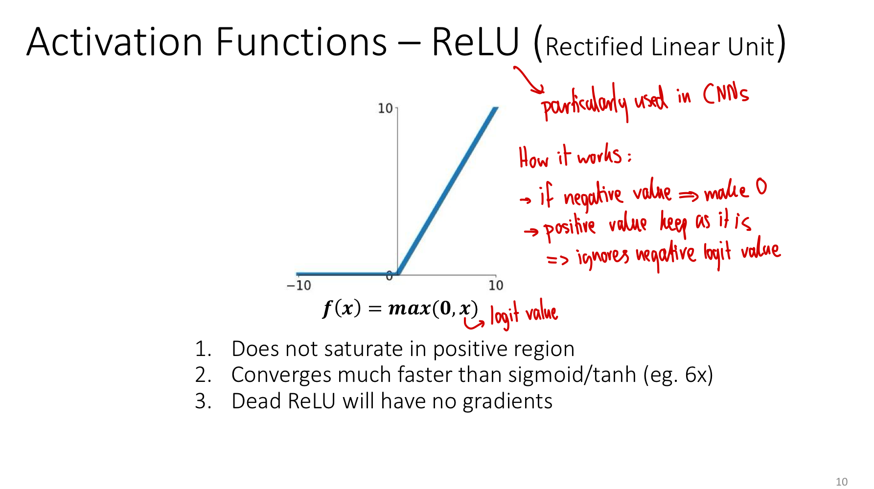
The rectified linear unit is dead simple: pass positive inputs unchanged, clip negatives to zero. Despite the simplicity (or because of it), this is the default activation for hidden layers in modern feed-forward and convolutional networks.

Why it works so well:

• No saturation in the positive region. For $z>0$, the gradient is exactly 1 — gradients flow undamped through any chain of active units. This is the single biggest reason ReLU networks train much faster than sigmoid networks (≈ 6× faster in the original AlexNet experiments).
• Cheap to compute. A single comparison and select, no exponentials.
• Sparsity. Roughly half of units are off (zero output) at any time, which has implicit regularisation effects and matches some biological intuitions.

The dying ReLU problem:

If a unit’s pre-activation $z$ is always negative for every input it sees, its output is always 0 and its gradient is always 0 — the unit is dead and never learns again. This can happen from a bad initialisation or a too-large learning rate that pushes a unit’s bias far negative.

In practice, dying ReLUs are usually a minority and don’t ruin training, but they motivate the next variant.

Leaky ReLU

$f(z)=\max (\alpha z,z),\alpha \approx 0.01$

Identical to ReLU on the positive side; on the negative side, output is a small fraction of the input rather than zero. The gradient is $\alpha$ (not zero) for negative inputs, so a unit can recover even if it temporarily produces negative pre-activations.

Trade-offs:

• Pro: No dead units. Doesn’t saturate in either direction.
• Pro: Same speed as ReLU.
• Con: Adds a hyperparameter $\alpha$. Empirically it doesn’t always beat plain ReLU on standard tasks.

There are further variants — PReLU (learn $\alpha$), ELU, GELU, Swish — each with their own justifications. ReLU and Leaky ReLU cover the basic intuitions.

Comparing them at a glance

Activation	Formula	Range	Saturates?	Zero-centred?	Notes
Sigmoid	$1/(1+e^{-z})$	$(0,1)$	Yes (both ends)	No	Output layers only
Tanh	$\tanh (z)$	$(-1,1)$	Yes (both ends)	Yes	Mostly historical
ReLU	$\max (0,z)$	$[0,\infty )$	No (positive); flat (negative)	No	Modern default for hidden layers
Leaky ReLU	$\max (0.01z,z)$	$\mathbb{R}$	No	No	Avoids dying ReLU

When to use what

The general modern recipe:

• Hidden layers in MLPs and CNNs: ReLU. Try Leaky ReLU if you suspect dead units.
• Output layer for binary classification: Sigmoid. Pairs with binary-cross-entropy.
• Output layer for multi-class classification: softmax (a generalisation of sigmoid). Pairs with categorical cross-entropy.
• Output layer for regression: No activation — output the raw $z$.
• Recurrent layers: Often tanh or sigmoid for gating, despite their saturation, because the dynamics need bounded outputs.

The vanishing gradient problem and depth

The story of the activation function is really the story of gradient flow through deep networks. In backpropagation, the gradient at a weight in layer $\ell$ is a product of factors, one per layer between $\ell$ and the loss:

$\frac{\partial L}{\partial w^{\ell }}\propto {\prod }_{k=\ell }^L{f}^{\prime }(z^{(k)})\cdot (\text{linear terms})$

If each $f^{\prime }(z)$ is bounded above by some value $\rho <1$ — as it is for sigmoid where $|{\sigma }^{\prime }|\le 0.25$ — then the product shrinks exponentially with depth. After 10 sigmoid layers, gradients are scaled by at most $0.25^{10}\approx 10^{-6}$ — well below floating-point noise. Early layers receive essentially no learning signal. This is the vanishing gradient problem.

ReLU sidesteps this: where it’s active, $f^{\prime }(z)=1$ exactly, so the gradient passes through undamped. Even if half the units are dead at any moment, the surviving paths carry usable signal arbitrarily deep. The shift from sigmoid/tanh to ReLU is a big part of why training networks deeper than ~10 layers became feasible in the early 2010s.

(Other ingredients matter too — better initialisation, batch normalisation, residual connections in week 5 — but ReLU is the foundational fix.)

Related

• sigmoid function — the canonical activation introduced in week 2; deep dive into its properties
• softmax — the multi-class generalisation of sigmoid for output layers
• backpropagation — the algorithm whose efficiency depends on the activation derivative being non-trivial
• multi-layer-perceptron — where activation choice between layers determines whether depth pays off
• convolutional-neural-network — where ReLU is the near-universal hidden-layer choice

Active Recall

Why must a multi-layer network use a non-linear activation? What goes wrong without one?

Composing linear maps gives a linear map: $W_2(W_{1}x+b_1)+b_2=(W_2{W}_1)x+(W_2{b}_1+b_2)$. Without non-linearity between layers, an $L$-layer network has the same expressive power as a single linear layer — depth buys nothing. The non-linearity breaks this collapse and lets each layer transform the representation in ways the previous layer couldn’t.

What is the "dying ReLU" problem, and how does Leaky ReLU address it?

A ReLU unit dies if its pre-activation $z$ is always non-positive — output is always 0, gradient is always 0, weights and bias never update. The unit is permanently inactive. Leaky ReLU replaces the zero output for $z<0$ with $\alpha z$ (small slope $\alpha \approx 0.01$). The gradient on the negative side is $\alpha \ne 0$, so the unit can recover from negative pre-activations and is not stuck.

Why does ReLU train networks much faster than sigmoid in practice?

Two reasons. (1) For positive inputs, ReLU’s gradient is exactly 1 — no saturation, no shrinking gradients with depth. Sigmoid’s gradient is at most 0.25, so gradients shrink by a factor of 4× per layer in the best case, exponentially worse with depth. (2) ReLU is a single comparison; sigmoid requires evaluating an exponential. Compounded over millions of activations and many epochs, the speed difference is significant (often quoted as ≈ 6× faster convergence).

A network has 20 sigmoid layers. Why might gradient descent fail to update the early layers' weights?

By the chain rule, the gradient at an early layer is a product of activation derivatives across all subsequent layers. Sigmoid’s derivative is bounded above by $0.25$, so the gradient is multiplied by at most $0.25$ per layer. Across 20 layers that’s $0.25^{20}\approx 10^{-12}$ — vanishingly small. Early layers receive effectively zero gradient and never learn. This is the vanishing-gradient problem; replacing sigmoid with ReLU largely fixes it because ReLU’s positive-region derivative is 1.

For each of the following, state the recommended activation: (a) hidden layer in a CNN, (b) output layer for binary classification, (c) output layer for 10-class classification, (d) output layer for predicting house prices.

(a) ReLU (or Leaky ReLU). (b) Sigmoid — output is interpreted as $p(y=1)$. (c) Softmax — outputs a 10-class probability distribution. (d) No activation — predict raw real-valued $z$ for regression.

What is sigmoid's derivative at $z=0$, and why is this the largest value the derivative ever takes?

${\sigma }^{\prime }(0)=\sigma (0)(1-\sigma (0))=0.5\cdot 0.5=0.25$. Since ${\sigma }^{\prime }(z)=\sigma (z)(1-\sigma (z))$ and $\sigma (z)\in (0,1)$, the product is maximised when $\sigma (z)=0.5$, which happens at $z=0$. In the tails, $\sigma$ approaches 0 or 1 and the product collapses toward zero — that’s the saturation that kills gradients.